By Adrien Debray, Johannes Lootens
Context
In 79 AD, Mount Vesuvius erupted, thousands of scrolls in a library located in a Roman villa in Herculaneum were carbonized by the heat of the volcanic debris. For centuries, as virtually every ancient text exposed to the air decayed and disappeared, these Herculaneum Papyri waited underground, intact.
The scrolls were discovered a few hundred years ago and have been waiting to be read using modern techniques. In 2015, Dr. Brent Seales was the first to read some scrolls without opening them using X-ray tomography and computer vision techniques.
Unfortunately, X-ray scans are not sufficient to read the scrolls as there is no clear contrast between the x-ray data of the carbon-based ink versus the carbon-based papyrus. It was however found out that machine learning models, trained on manually annotated fragments could pick up subtle surface patterns in the X-ray scans indicating the presence of ink on the papyrus.
Therefore, Dr. Brent Seales and his team asked for help to the ML community by launching the Vesuvius Challenge. This challenge offers a $700k grand prize to the first team able to read the Herculaneum Papyri. A big part of this challenge consist of being able to detect ink on 3D X-ray scans of detached fragments. Because it is possible to extract ground truth data of the ink on the fragments, the Ink Detection Progress Prize has been launched on Kaggle.
Aim of this post
Artificial neural networks are commonly used for segmentation task using 2D images data as training. The ink detection challenge is particular as it is a semantic segmentation problem using 3D (X-ray scan) data. There is not a lot of scientific literature available to assess the performance of neural networks for this type of problem.
The purpose of this post is to further explore this problem, discuss our approach, elaborate on specific model architectures, possible preprocessing, etc. and see how these perform on this specific use case.
Data
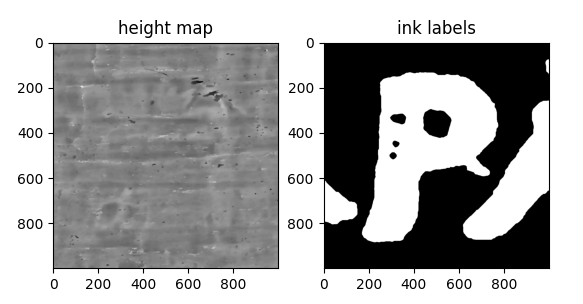
The training data available for the Ink detection challenge consist of three broken-off fragments of scrolls that were opened physically (and destroyed in the process). To generate labels, these fragments where photographed and later ink was annotated manually on the resulting infrared images.
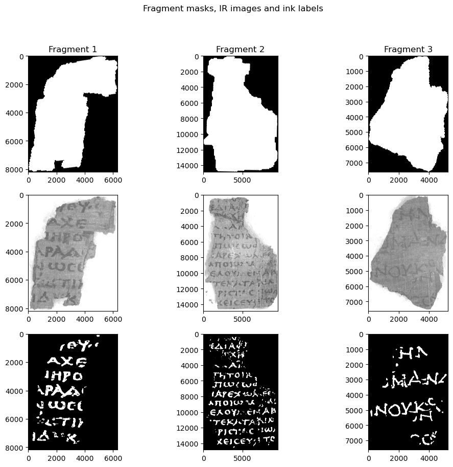
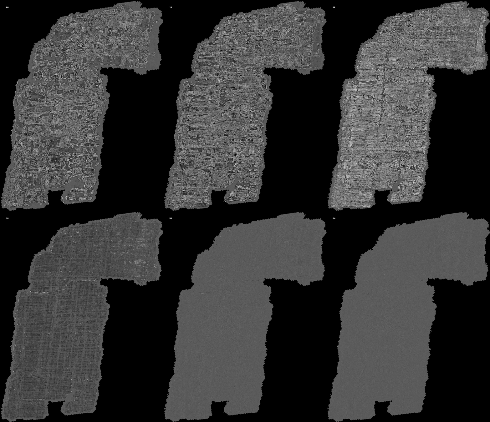
Since the goal is to be able to read ink from the digitally unrolled scrolls, the data available for inference consists of just the 3D X-ray scans of the fragments without any IR images. And unlike on the IR images, the ink is not immediately visible on those. However, experiments have shown that it is possible for a trained ML model to indirectly detect the ink anyway.
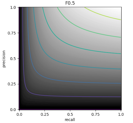
The actual training objective is to generate a 2D, binary mask for a test fragment where a 1 indicates a pixel with ink. To evaluate this the F0.5, metric is used

This is a variant of the F1 metric that values precision higher than recall since this results in more readable letters in this specific use case.
Challenges
This section will briefly discuss the main challenges in this competition.
Data set size
A first big challenge is the limited amount of training data. The train set consists of only three different fragments with sizes ranging from approximately 8000x6000px to 14000x8000px. Or about 3500 patches of 256x256px. However if you increase the patch size to 512x512px or even 1024x1024px, the amount of training samples is reduced to around 900 or 225 respectively. Additionally, these fragments are not perfectly rectangular so this still includes quite some completely empty crops in the border of the images. So, while normally increasing crop sizes would be an easy way to increase performance, this is made much more challenging here as the model will be much more prone to overfitting and would require robust regularization to compensate for this.
3D data
A much more interesting challenge is the actual shape of the data. While the goal is to generate a 2D mask, the data used to generate this is very much three dimensional, consisting of an X-ray scan with 65 layers. Additionally, since the ink is not clearly visible in X-ray data and has to be identified indirectly in slight changes in texture, surface height, … resulting in the information about the ink being located in “roughly” the upper half of the papyrus. Since the height of the papyri also varies significantly both within and between fragments, one can’t simply select a few layers to greatly simplify the problem but does actually have to take the 3D structure into account.

Vertical cross-sections of the X-ray data. The images on the left are slices along the x-axis, images on the right are slices along the y-axis
As a result one has to either use 2.5D or 3D segmentation approaches. Additionally, every operation suddenly becomes much more memory-hungry since all images now have up to 65 channels instead of the usual 3 for RGB images or just 1 for grayscale images.
Approach
Here the approach we took to solve the challenges previously mentioned challenges will be discussed. Starting with the model architecture used, attempts to flatten the data, followed by regularisation, optimizing inference and finally a quick recap of the final solution.
U-net Architecture
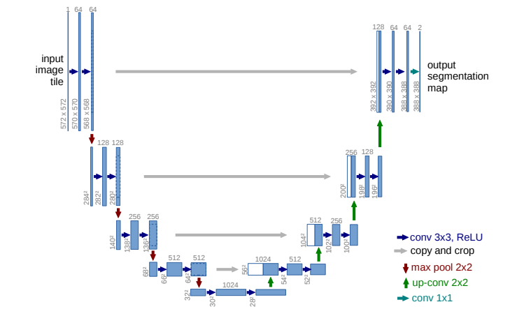
The U-net architecture contains an encoder part to extract the relevant features from the image and a decoder part to build the segmentation mask from these features. This is found to be very effective for semantic segmentation tasks where each pixel of the input image needs to be classified. Moreover skip connections are used to add feature maps from the encoder to the corresponding decoder layers which brings high-resolution information that might be lost in the downsampling layers. You can refer to the research of Ronneberger et al. for more information about UNET’s.
3D vs 2.5D CNN segmentation
To handle the uncertainty and variability of in which slices the ink is located in the 3D X-Ray data of our fragments, 3D and 2.5D CNN (convolutional neural network) segmentation methods are explored.
3D CNN model
In 3D CNN, the input is a full 3D volume. The convolution kernels used have 3 dimensions and thus spatial relationships between neighbouring slices are captured. The exact model implemented here is a 18 layers ResNet model. The structure of the ResNet 18 contains 4 layers of 2 basic blocks, each block consists of two 3D convolutions. A skip connection is added between every block in order to let the gradients flow directly backward to initial filters. More info about ResNets can be in this blogpost.
2.5D CNN model
The input data in 2.5D CNN is a set of 2D slices extracted from the 3D volume, each slice is treated as an individual input by 2 dimensional convolution kernels. The outputs of each slices are then combined to generate the final prediction. The exact model implemented here is a U-net architecture, using the EfficientNet b0 backbone as an encoder, from the segmentation models library for PyTorch.
Baseline scores for these two models can be found in the table below:
| Experiment | Crop Size | Z-channels | validation F0.5 |
|---|---|---|---|
| Resnet18 - 3D baseline | 256 x 256 | 24 - 40 | 0.56 |
| Efficientnet - 2.5D baseline | 224 x 224 | 29 -34 | 0.51 |
Overall the 3D Unet was found to outperform the 2.5D version. This was not a very big surprise with lots of the information about the ink being distributed throughout multiple layers. One idea was to flatten the fragments (as discussed below) to mitigate this problem but without much success.
Flattening the fragments
One idea to decrease the complexity of the problem (and the network required to solve it) was to flatten the fragment and focus on only a few layers, greatly reducing the complexity of the problem by eliminating variables that don’t contribute in the lower layers of the papyrus and the air above the fragments.
To this end, several classical computer vision segmentation techniques were tried to segment the papyrus from the air (a full comparison can be found in this notebook). A deep learning approach would probably have performed better but there were no labels available to train this.
After some experimenting, using a Sobel filter over the Z-axis, thresholding and taking the argmax resulted in the most robust solution in most cases. This also had the added advantage of being a “memory friendly” solution (unlike KMeans and DBSCAN). All classical CV techniques were found to be very sensitive to noise so denoising the fragment beforehand with the help of a Gaussian filter proved essential.
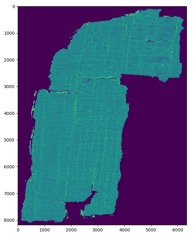
Three different approaches were tried for incorporating this height information into the training data of the 2.5D baseline:
- Add the height map as an additional channel, resulting in a model input consisting of 6 intensity channels (z-layer 29-34) + 1 height map channel.
- Use the height map to flatten the training data and take the top 6 layers of the flattened papyrus, with one air layer as a buffer as model input.
- See 2. but also include the height map channel as input, for a final input of 7 layers, to reintroduce any height information that was lost.
Despite the idea sounding nice in theory, either the quality of the height map was not sufficiently accurate or the loss in texture/height information outweighed the advantage of having a better cross-section.
| experiment | Model input | # channels | validation F0.5 |
|---|---|---|---|
| baseline | cross-section (29-34) | 6 | 0.51 |
| 1. | cross-section (29-34) + height map | 7 | 0.49 |
| 2. | flattened cross-section | 6 | 0.50 |
| 3. | flattened cross-section + height map | 7 | 0.50 |
Handling overfitting
When trying to increase the crop size that the model uses, it started overfitting noticeably more since doubling the size of the crop side results in 1/4th the amount of training samples. Due to the already limited amount of training data this makes a very big difference. As such robust regularization is needed to offset this.
*All experiments below show the results of a UNet with a 3D resnet as backbone, trained on crops of 512x512 px.
1. Augmentation
A first way to increase regularization is to increase the amount of training data. Specifically generating new samples using augmentation.
For augmentation, transforms from the Albumentations package was used and the list of used augmentations can be found below.
| augmentation | p | Description |
|---|---|---|
| HorizontalFlip | 0.5 | Flip the image over the y-axis. |
| VerticalFlip | 0.5 | Flip the image over the x-axis. |
| ShiftScaleRotate | 0.75 | Randomly apply a translation, scaling and rotation of the image. |
| CoarseDropout | 0.2 | Randomly introduce a hole in the image. |
| ChannelDropout | 0.2 | Randomly drop a channel from the image. |
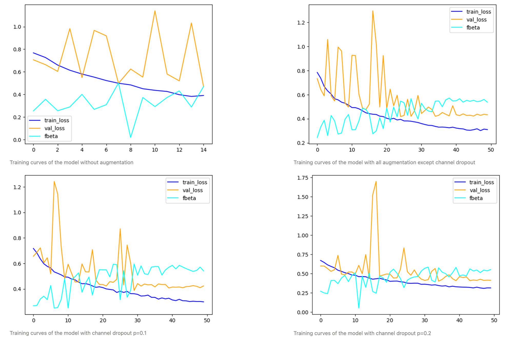
When comparing experiments with different amounts of augmentations, it becomes clear how important it is for this use case.
While the model with a channel dropout of 0.2 clearly generalizes the best, the one with a slightly more conservative p=0.1 for channel dropout generally yields slightly higher optimal F0.5 scores but is calibrated worse.
| experiment | epoch | train_loss | val_loss | thresh | F0.5 |
|---|---|---|---|---|---|
| no augmentation* | 8 | 0.50 | 0.50 | 0.75 | 0.50 |
| no channel dropout | 23 | 0.33 | 0.42 | 0.8 | 0.57 |
| channel_dropout 0.1 | 30 | 0.36 | 0.39 | 0.9 | 0.61 |
| channel_dropout 0.2 | 32 | 0.36 | 0.42 | 0.55 | 0.58 |
2. Dice loss
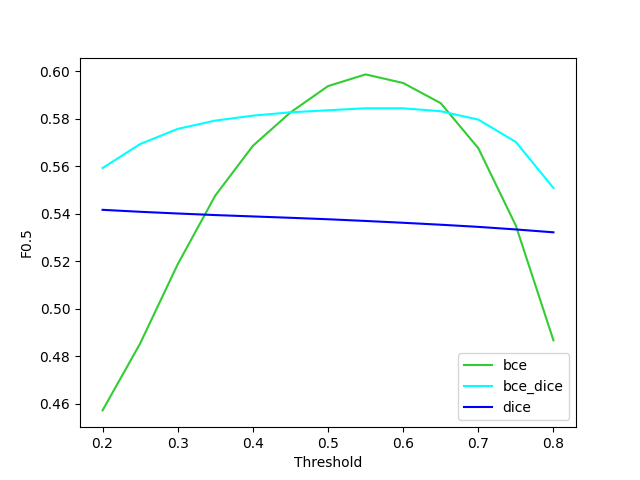
A second way to have a more robust model is not to just use binary cross entropy, but DICE loss (2(p∩gt)/(p∪gt)), as well. This loss was designed specifically as a loss function for highly unbalanced segmentations. Using this loss does lead to a model that is much less sensitive to the threshold but does have a lower optimal F0.5. Using an average of the two leads to a model that has a slightly lower optimal F0.5 but is much more robust to not having an optimal threshold.

Optimize Inference
Once inference is made, a quick win could be to handle the predictions our model is making. Several techniques were tried using knowledge in order to get better and more robust results.
1. Test Time Augmentation (TTA)
TTA applies different transformations to the test data, to feed these transformations in the trained model and then aggregate (usually by averaging) the results to get a final prediction. Providing the model multiple perspectives on the same image and averaging the prediction will make the inference more robust and reliable. The TTA performed here rotated the input images 4 times by 90°, making inference time significantly longer, but improved the LB by more than 0.1 in most cases.
2. L1 / Hession Denoising of the predictions
This idea proposed by Brett Olsen during the competition (Improving performance with L1/Hessian denoising)
The approach here is to make use of known properties of the ink distribution:
- The ink is sparse, most regions will not contain ink. We can add a L1 regularization term to the predictions to penalize noisy data.
- The ink is continuous, a single pixel is more likely to contain ink when it is next to another pixel containing ink. A Hessian matrix term is used to penalize strongly variable values of ink/no-ink.
Adding denoising to the output increased inference time by a bit, while raising the LB score by an mostly insignificant amount
| TTA | Denoising | Inference Time | Public test F0.5 | Private test F0.5 |
|---|---|---|---|---|
| yes | no | 1h27 | 0.57 | 0.51 |
| no | no | 19 min | 0.44 | 0.35 |
| yes | yes | 1h32 | TODO | TODO |
Final Solution (kaggle notebook)
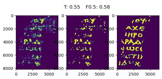
Our final solution consists of a UNet with a 3D Resnet as backbone, trained for 32 epochs, with a combination of BCE and DICE loss, on fragments 2 and 3 (the final model was not retrained on the complete train set due to running out of GPU time). While this was not the model with the highest F0.5 on the validation set, it is the one we trust to generalize the most, which is especially important with the hidden test set. At inference time, test time augmentation is used (inference is performed on images rotated 0, 90, 180 and 270 degrees and the average of these is used as the final prediction) and the prediction masks are denoised in order to remove any small blobs that are extremely unlikely to be ink. The final validation and test scores can be found below together with the final prediction for the validation set.
| threshold | validation F0.5 | public test F0.5 | private test F0.5 |
|---|---|---|---|
| 0.55 | 0.58 | 0.57 | 0.50 |
Other ideas that could have improved performance
While not currently present in our final solution, there are still some things that could be done to improve the result. In this section you can find a list of things that would most likely improve performance/ be interesting to look at/ …
Ensemble
A not very interesting but very reliable way to improve performance is to just take a bunch of your best performing models and instead of just using the best, use all of them and aggregate the predictions (usually by taking the mean) to end up with a more robust solution. If you want to squeeze the most out of your existing work this is definitely the way to go.
Thresholding strategy
In our current solution the threshold used was decided by finding the threshold that yielded the best F0.5 for the validation set. This does requires a validation set to decide this optimal threshold and, depending on the variance of the model, can lead to overfitting to this validation set. While some models with a lower variance were calibrated slightly better and were much more robust to a slight change in threshold, these often had a lower optimal F0.5 score. As such, a reliable thresholding strategy could lead to a decent increase in performance.
Overlap-tile strategy
Some artefacts are clearly visible at the edges of the crops. To prevent this ideally one would only use the centers of the predicted patches this is also mentioned in the original Unet paper where they use it for “seamless” segmentation.
Transformer based segmentation approach
Recently, transformers have been revolutionizing a variety of ML fields and this includes semantic segmentation. Here, models such as SegFormer, Swin Transformer and Mask2Former for 2D images and UNETR in 3D have been dethroning the classical CNN based approaches for quite some time now. It would have been interesting to see how they perform here.
Conclusion
In conclusion, we highlighted in this blog post our approach for the Ink Detection Progress Prize launched on Kaggle. The aim was to further explore this unusual challenge and show insights on questions regarding the models performances on this type of 3D data, if effective preprocessing can be done …
Our approach was data-centric. We prioritized performing a strong exploratory data analysis (EDA) to understand the challenges before training numerous models. These came mainly from the 3D shape of the data, X-ray scans of 65 layers made every operation much more memory-hungry, and the small dataset size, only 3 fragments. Fragment flattening was tried to simplify the problem and, while looking promising at first, did not do much in the end. Instead working with a 3D model that was able to extract as much information from the different layers proved to be the approach that yielded the best results. However this approach needed much more regularization to work properly. To limit overfitting; data augmentation, especially channel dropout and training using a combination of the BCE and DICE losses increased the F0.5 score considerably and led to a more robust model.
Since we only started 2 weeks before the deadline, had access to limited GPU time (30h/week/person) and infrastructure (15 GB of GPU memory) we were prevented from training and tuning all the models we wanted so we limited ourselves to exploring a limited selection in depth. However, the U-net architecture showed, as expected, to be very performant for pixel-level segmentation. The Resnet18 backbone with 3D convolutions has already shown decent results compared to the top of the leaderboard of the competition, where much of the remaining performance gap lies in training deeper models on larger crops (with proper regularization) and selecting those to generate a final ensemble. Nonetheless we would definitely recommend the discussions on Kaggle of the competition winners as literature.
We hope you gained useful insights about this challenge reading our blogpost. You can find all our code explained in a comprehensible way in notebooks on our Github repo. Do not hesitate to take a look and try to improve the results yourself, all is explained there!
Lastly, we participated in this competition and wrote the blogpost as a team with our Dataroots colleagues. We would like to express our gratitude to Cynthia Laureys and Vitale Sparacello for their guidance, and to Zoë Van Noppen and Omar Safwat for their contribution to the ideation and the launch of this initiative.


