

By Warre Dreesen, Martial Van den Broeck
Detecting drift in your data is very important when deploying models in production. It ensures that the performance of your model does not decrease due to the nature of the input data changing. There are a lot of tools out there for monitoring your data and detecting drift such as Great expectations, NannyML,... . However most of these are made for tabular data. In this blogpost we will discuss different approaches for detecting drift in images using popular tools.
Creating drift using data augmentation
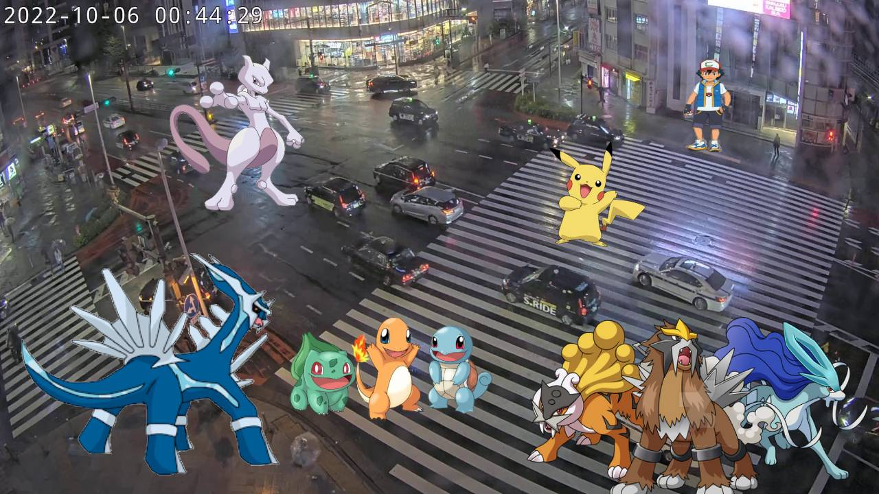
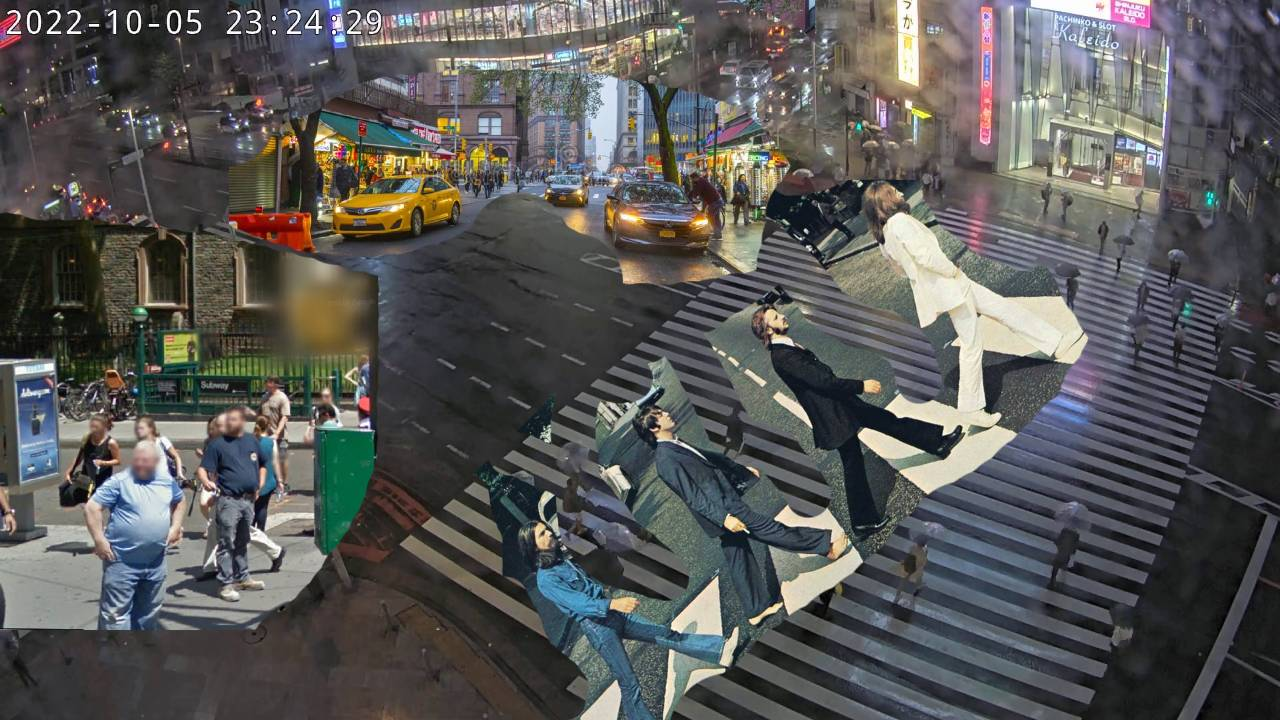
To create drift we took on two different approaches. The first approach was to create one-shot images that are clearly outliers. These images were created by Silke and resulted in what can only be called art.
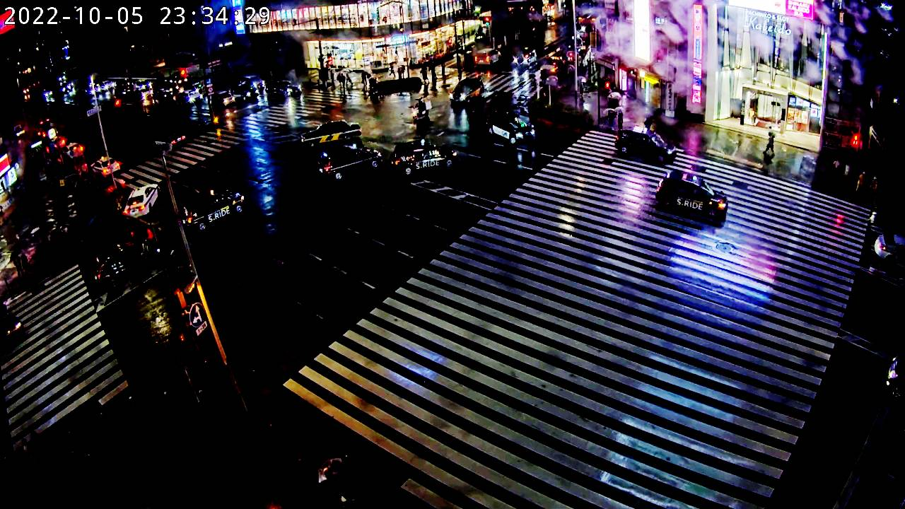
As a result the crossroads of Tokyo have never been so unsafe. In a span of one night it saw Romans attacking, Dragons lighting fire and for some moments they transcended to dimensions unheard of. However, the model should not be retrained on glitches of alternate realities, thus should be discovered before they establish a spot in the dataset used for retraining!

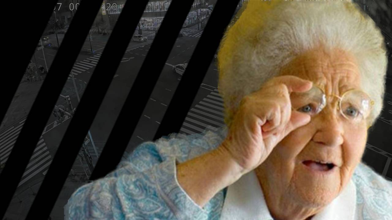
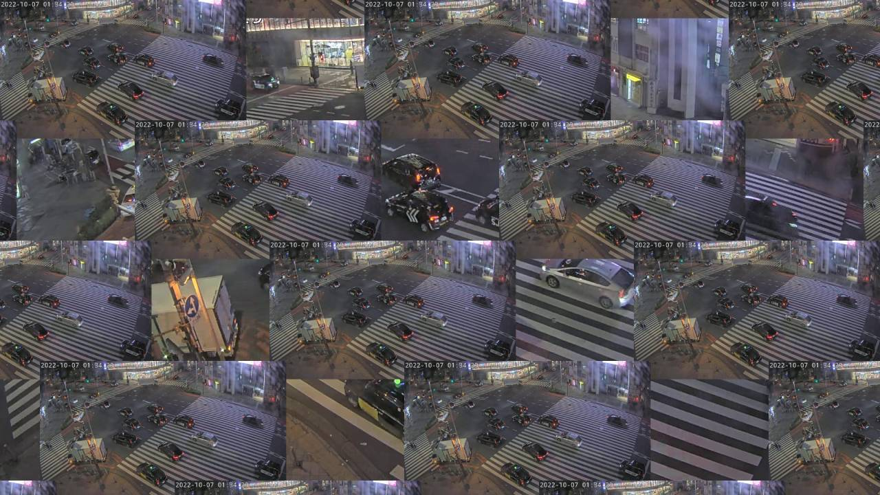
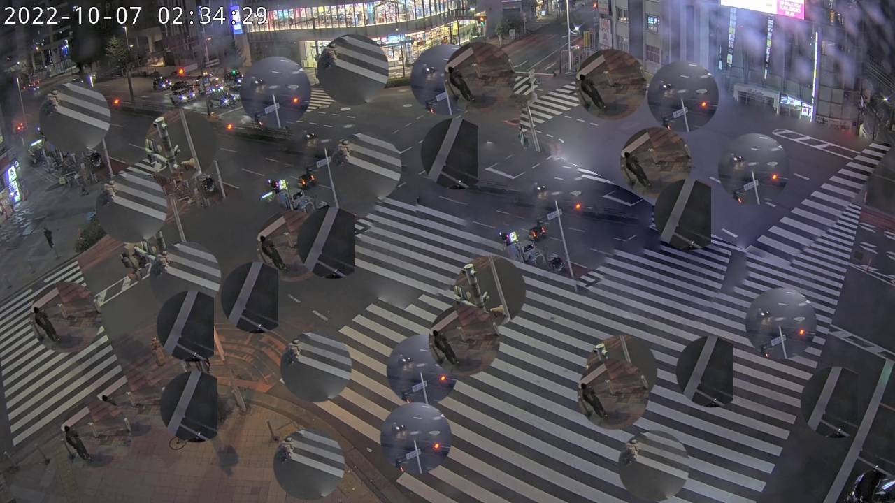
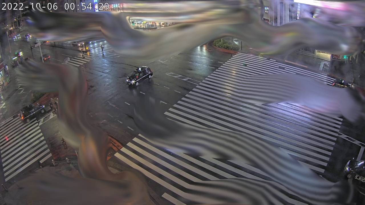
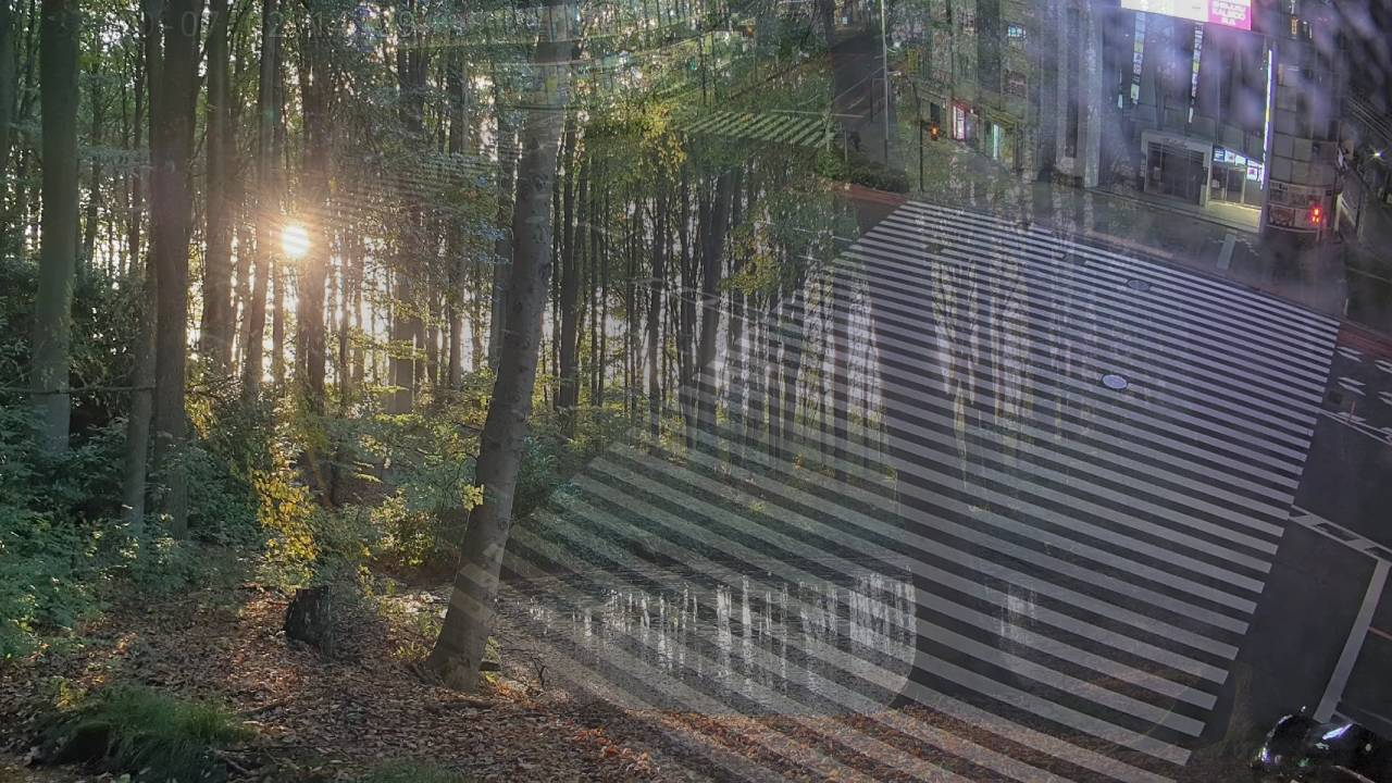
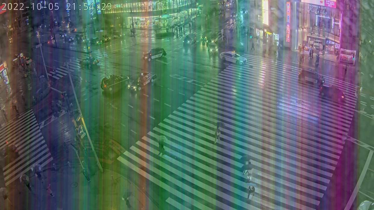
Our second approach was a more automated one. Here the idea was to try out an image augmentation library, Albumentations, and use it for adversarial attacks. This time, instead of one-shot images, we applied the transformations at random time ranges. We chose for these transformations also to be more subtle than then one-shot images, such as vertical flips, grayscaling, downscaling, …
The overall use of the package is very easy. The Albumentations library comes with different transformations that can easily be applied to pictures. These transformations go from simple adjustments such as a vertical flip to inserting rain into the pictures.
They also provide a way to easily chain different transformations into an image transformation pipeline. This pipeline object can then be used whenever you want this set of transformations to be applied to a picture.
transform = A.Compose([
                        A.VerticalFlip(p=1),
                        A.ToGray(p=1),
      		])
transformed_image = transform(image=original_image)["image"]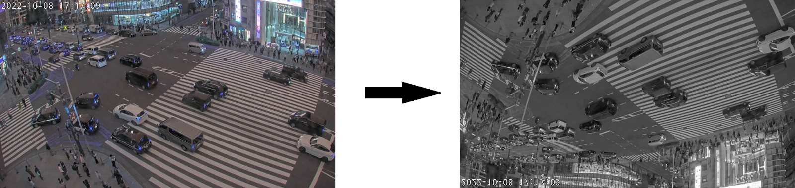
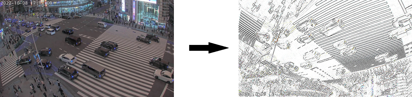
Although Albumentations comes with a list of transformations, it is likely that not all transformations you’re looking for are there exactly in the manner you’d want them. Luckily it is pretty easy to include transformations from different libraries (or your own written ones) in the transformation pipeline by inheriting from Albumentations ImageOnlyTransform class.
 class MyTransformation(ImageOnlyTransform):
    @property
    def targets_as_params(self):
    	return ["image"]

    def apply(self, img, **params):
		# Example of a transformation defined by ourselves
    	sobelxy = cv2.Sobel(src=img, ddepth=cv2.CV_64F, dx=1, dy=1, ksize=5) # Combined X and Y Sobel Edge Detection
    	inverted_sobelxy = 255 - sobelxy
    	return inverted_sobelxy

    def get_params_dependent_on_targets(self, params):
    	img = params["image"]
    	return {}
Which we can then use in our transformation pipeline
my_transform = A.Compose([
                            MyTransformation(),
                            A.VerticalFlip(p=1)
				])
This way we defined 10 different ‘more subtle’ transformations, in which we applied the transformations to different periods of time within the span of a few days. The test would be whether the drift detection would be able to detect these transformations.
We’re expecting that transformations that have no abrupt change in the color scheme will be harder to detect, especially when working with metrics such as hue, saturation and brightness. Following this logic it would be interesting if the models can spot the following transformations:
Distortions:
- Vertical flip
- Downscaling
- Adding Rain
- Gaussian noise
- Emboss
Color based:
- Color jitter
- Inversion
- Grayscale
- Sunflare
- Shuffling color channels
Although the use of Albumentations is a breeze, their transformations were not always well documented and for an image augmentation library lacked in, well, images...
It would be great to see an example for the different transformations, without having to test them all out in code to see how they look.
From images to tabular data using Resnet
Since most popular monitoring tools make are designed for working with tabular data our goal is to split the task up in two parts. First we try to extract features from the image that can be stored as tabular data. This then allows us to use the already existing technologies for detecting drift on this tabular data that was created.
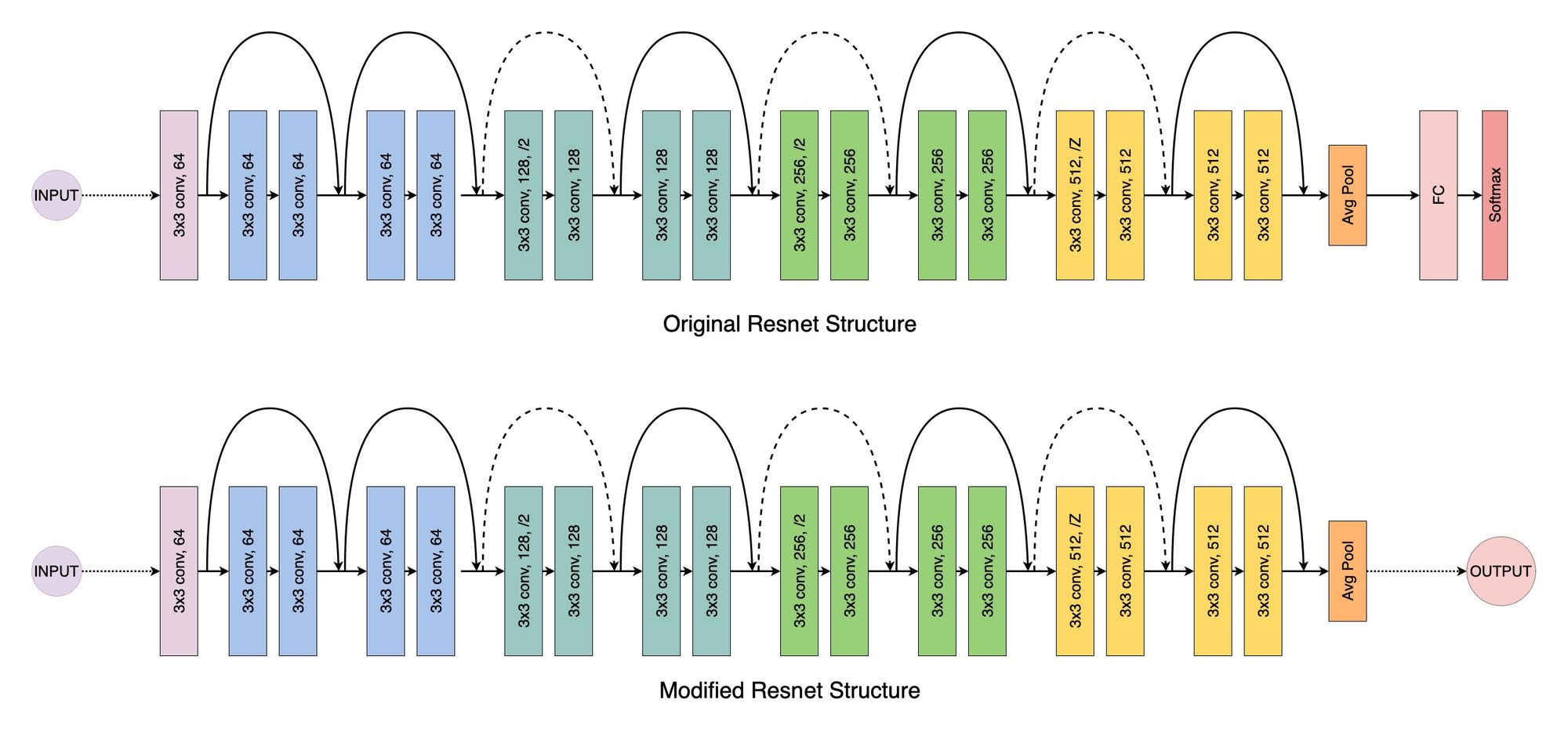
For the extraction of features from the images we used a pretrained Resnet18 model that was trained on Imagenet1k. In order for it to be usefull for our usecase we removed the last fully connected layer containing the class labels and took the output of the Avg Pool layer as our features. The 512 features obtained from the resnet are then further reduced using PCA. This results in the final tabular dataset with 150 features for each image.
NannyML to detect datadrift
Now that we have converted the images to tabular data it is possible to use popular tools on it to detect data drift. NannyML is able to detect complex and multivariate changes in the input data by using data reconstruction with PCA. First a PCA-transformation will be fitted on the training data that tries to capture the distribution and properties of the data.
Secondly the train data will be compressed using the PCA-transformation and then immediately reconstructed with the inverse PCA-transformation.
Lastly the euclidian distance between this reconstructed image and the original image is computed. This distance is called the Reconstruction error and is used as a one-dimensional metric to classify drift. By thresholding this error it is possible to distinguish drifted images from regular images.
In the figure below you can see that there is a shift in the reconstruction error between images that the resnet was trained on and unseen images even though these unseen images are very similar and should not be detected as drift. To solve this problem the training set is split into 2 parts. One to train the resnet and another one to determine the correct threshold for the reconstruction error.

In our implementation the dataset is split in three groups of images. A training set that is used to train the Resnet, a validation set that is similar to the training set but that is not seen during the training of the Resnet and a test set consisting of drifted images and healthy images.
The figure below shows the distribution of the reconstruction error for the different groups. This figure shows that the Resnet approach is able to separate the different distributions and allows for drift in the images to be detected.

Why logs
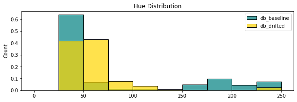
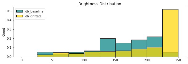
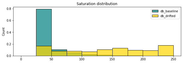
Instead of using the computationally expensive Resnet to convert the images to tabular data it is also possible to use Whylogs. The good news with Whylogs is that the tool supports images. Indeed, there is a function allowing to create a statistical profile of an image batch based on saturation, hue, brightness or even width and height of pixels.
The purpose is then to compare the distribution of those different features between our images and a potential drifted image. A first step is to visualize the distributions through the use of histograms.
The question is how to use the distribution of several features to define if an image is drifted or not ? We could use the mininum and the maximum as threshold and categorize an image as drifted if its profile doesn't stand in this range. This approach is trivial and percentage of detection is very low. Indeed, even in our small examples, it wouldn't have detected anything while the distribution are very different.
Fortunately there exists metrics to compare distributions and histograms and we will use two of them, the Kullback-Lebler divergence and the histogram intersection.
Even if KL divergence is not a true statistical metric of spread as it is not symmetric and does not satisfy the triangle inequality, it is easy to calculate and gives decent results. Concerning the histogram intersection, it measures the area of overlap between the two probability distributions. A histogram intersection score of 0.0 represents no overlap while a score of 1.0 represents identical distributions.
Performance comparison
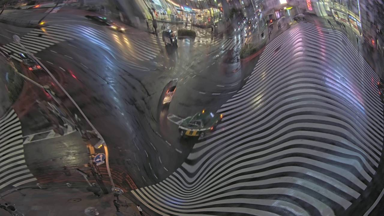
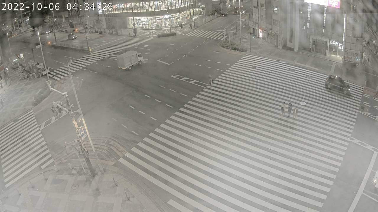
To test the performance of these methods we worked with a dataset of images from a crossroad in Tokyo. It consists of 635 images and to these images 55 outliers were added. The outliers range from some subtle drift in the image to not so subtle photoshops as seen in the picture below.
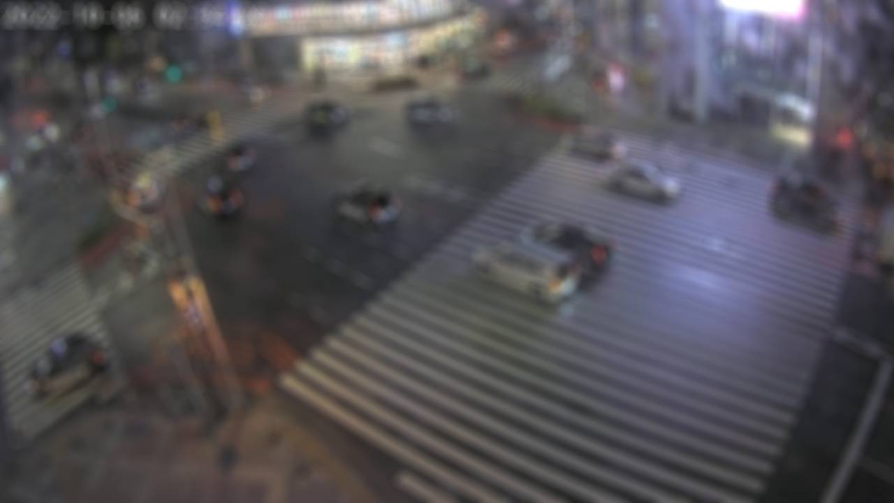


In order for us to be able to compare the different methods we split the dataset into a training set of 400 images and a test set of 235 images to which the 55 outliers are added for a total of 290 test images. the precision and recall of the two approaches is shown in the table below.
| MODEL | Precision | Recall |
|---|---|---|
| Resnet + PCA | 96% | 93% |
| Whylogs | 91% | 80% |
The Resnet +PCA approach is able to detect more of the drifted images and also has a higher accuracy with its predictions than the Whylogs approach. Let's dig a bit deeper into which images are and are not detected.
Let's start off with the Whylogs approach. It's very lightweight and tries to detect the drift based on brightness, hue and saturation. Therefore it detects most of the drifted images that have a large change in color such as flames or Pokemon with bright strange colors. For this dataset this simple and lightweigt approach results in decent performance considering that the computational cost is rather low.
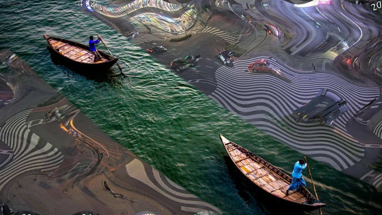
The Whylogs approach however does struggle with images were there are strange shapes present, but the color doesn't change that much. This is visible in the images it missed that are shown above. In these images the drift is happening by changing the shape of the images instead of changing the colors. Luckily the Resnet approach doesn't suffer from this.
The results showed that the Resnet has better performance than the Whylogs approach. However it does come with a greater computational cost that can be the difference maker for eventual use-cases.
While the Resnet approach is very good at finding strange shapes and objects it still struggles with a certain kind of images. In the distributions of the reconstruction error we can see that there are a small number of images very close to the decision border. These images all have drift applied to them related to a change in brightness or color.
Apart from the color images there is 1 other drifted image that is not detected by the Resnet approach. It is that small blue box in the histogram with a reconstruction error of only 11. It is a cow on the loose.
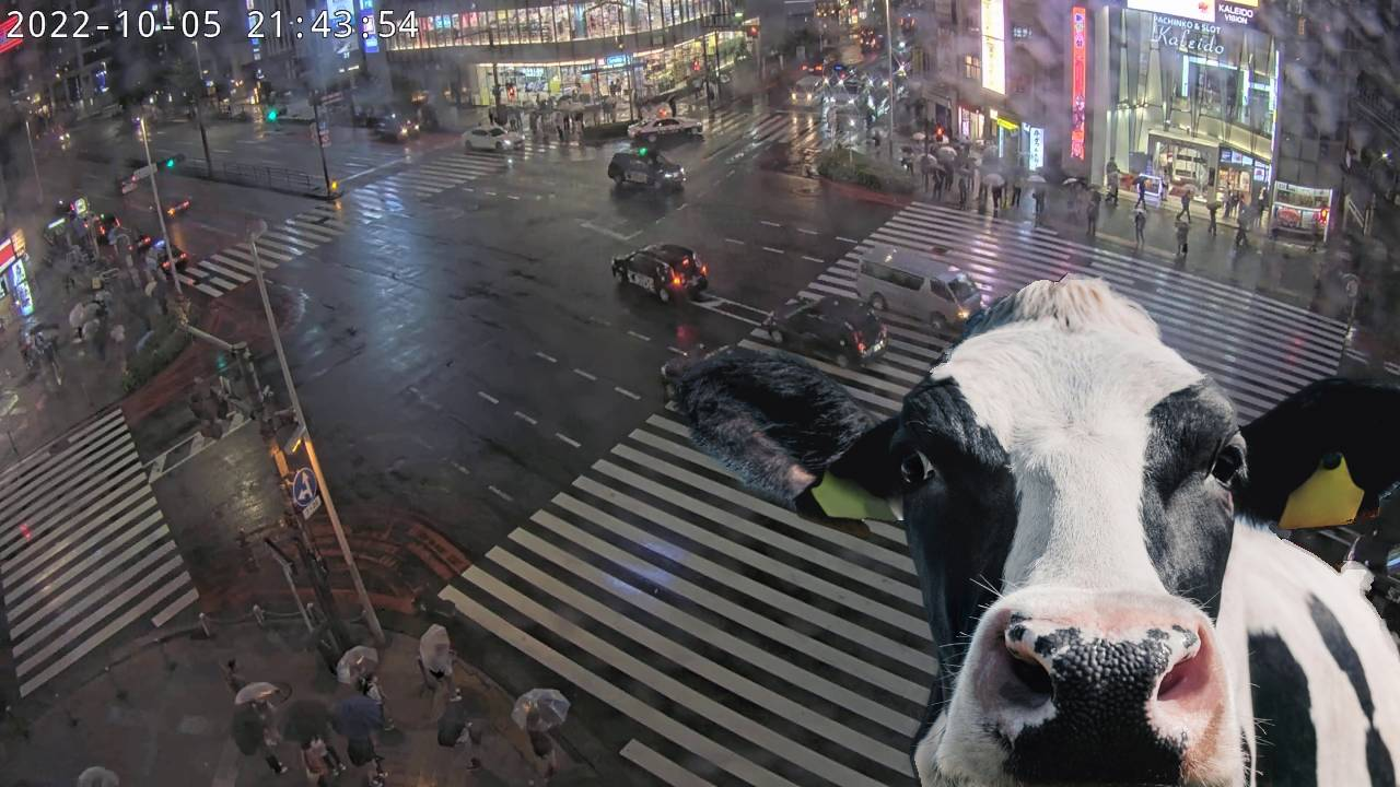
Despite the Resnet approach being very good at detecting strange shapes or objects it doesn't detect this strange cow. Why it doesn't detect it? We have not dug deeper into the data to understand the and fine tune the approach.
Luckily this escaped cow is easily detected by the Whylogs approach so there is no need to panic.
Conclusion
This blogpost was one big adventure filled with mythical creatures, crazy streets and a cow? But it most importantly showed that drift detection is not only possible for tabular data but that it can also be used for images. Both the approaches have clear advantages and disadvantages.
The Resnet while computationaly expensive provides great performance and is able to detect almost all the drifted images. However it struggles when the drift is only applied to the color space and not to the shapes in the image.
On the other-side we have the Whylogs approach which is very lightweight and bases it's decision almost completely on colors, brightness and saturation. While being lightweight the performance is still comparable to the Resnet approach. But it does struggle detecting drifted images containing unusual objects.
Luckily the two methods complement each other perfectly. The weak points of one method are the strong points of the other one.