Statistics Saga 2: Dimensionality Reduction

Welcome back! If you remember from last time I told you we would continue with matrix factorisations, more specifically dive into some dimensionality reduction techniques! Hope you're ready!

This blogpost will give you a comparison of two specific factorisation techniques that are foundational to the idea of dimensionality reduction: principal component analysis and factor analysis.

Some of the techniques are also given some context with examples from a recent psychology study. Which is a bit more fun than the billionth iris flower dataset example. At least we think so!

Dimensionality reduction

Dimensionality reduction, the term leaves very little to the imagination: techniques that can reduce the dimensionality of data. Why is this useful? We live in a 3 dimensional world, higher dimensional relationships are very difficult for us to reason about. The relationship between the height and weight of a person is not too difficult to think about, it only uses 2 dimensions. Include age into this relationship and we start to struggle a whole lot more. Similarly, computers can also struggle with high dimensional data: calculations and models become a lot less efficient.

💡

psychology example
Within the field of psychology dimensionality reduction is often used when dealing with multivariate data. Usually this is done to infer or measure latent/unobservable traits. As an example: psychologists have long attempted to characterise what an emotion is. One of the first ideas, and it has stuck around, is that at the very least an emotion should have two properties: valence and arousal. The valence of an emotion is how pleasant or unpleasant it is. You can think of it on a spectrum of the happiest a person could ever be to the saddest a person could ever be. The second property, arousal, is perhaps a bit less straightforward. You can think of it as how much an emotion activates you. If you’re extremely angry or happy you’re in a high arousal state, while boredom or feeling at ease would be a low arousal state. An intuitive next step might then be to conceive of any emotion as a combination of some arousal and valence on a 2D-plane.

stop for a moment and think about how you are feeling right now.
Happy 1 - 2 - 3 - 4 - 5
Sad 1 - 2 - 3 - 4 - 5
Bored 1 - 2 - 3 - 4 - 5
Miserable 1 - 2 - 3 - 4 - 5

The amount of emotions a person would have to rate could vary, but is usually at least 10 items. A matrix factorization model is then applied to the gathered data. Reducing the dimensionality of the data to only 2 dimensions would reflect the underlying levels of valence and arousal.

For this reason dimensionality reduction is used in machine learning to combine a set of variables into a smaller set and use this smaller set as features for a model. This can be beneficial when dealing with a huge amount of features because it reduces the space in which the model has to find solutions. However, there are downsides to doing this. Firstly, you are throwing away information. While ideally only statistical noise is discarded, these techniques all make some assumptions about the structure of the data. If these assumptions do not hold useful information might get excluded from the model. Secondly, when combining multiple features into one, model explainability is negatively impacted. It is much harder to interpret a regression coefficient for a feature that is combination of 10 other features than it is to individually compare those coefficients. That is to say, one should carefully consider the up- and downsides when applying dimensionality reduction. Thoroughly research the algorithm or model you wish to use, taking into account the specific question or problem you wish to address.

Having introduced and explored the basic ideas behind dimensionality reduction we’ll next compare and contrast two different techniques, Principal Component Analysis (PCA) and Factor Analysis (FA). PCA is a very popular technique used in both machine learning and statistics. FA is a less popular technique that has its origins in psychology/psychometrics. Why FA then? The techniques are very similar, as we shall see, and serves to illustrate how small changes in a model can make it more or less appropriate given a specific task. Also, the author of this blog is a psychometrician who has no qualms with picking their favourite child.

PCA and FA

Let’s first look at how an FA is defined so that we may compare it to PCA and understand the differences. Factor analysis as a model of our data can be specified as:

$$ X = \Xi \Lambda' + \Delta, $$

where $ X $ is our observed data, with $ n $ observations and $ p $ variables. $ \Xi $ is a matrix of factors with dimensions $ n $ and $ m $ where $ m $ ≤ $ p $. $ \Lambda' $ is a $ m $ x $ p $ matrix of factor loadings or weights. Lastly $ \Delta $ is an $ n $ × $ p $ matrix of error terms.

Now, let’s refresh our memory on PCA, which is usually defined as follows:

$$ X = Z_s D^{1/2}U'. $$

$ X $ is again our observed data, $ Z_s $ the standardized principal components, $ D^{1/2} $ a diagonal matrix of the standard deviations of the principal components, and $ U' $the matrix of eigenvectors. What we are doing here is a singular value decomposition of the observed data matrix.

If we apply these techniques to a covariance matrix, the difference becomes clearer. Let’s call this covariance matrix,

$$ R = \frac{1}{(n-1)}X'X $$

which we’ve calculated using some of the emotion data mentioned in the previous example [1].

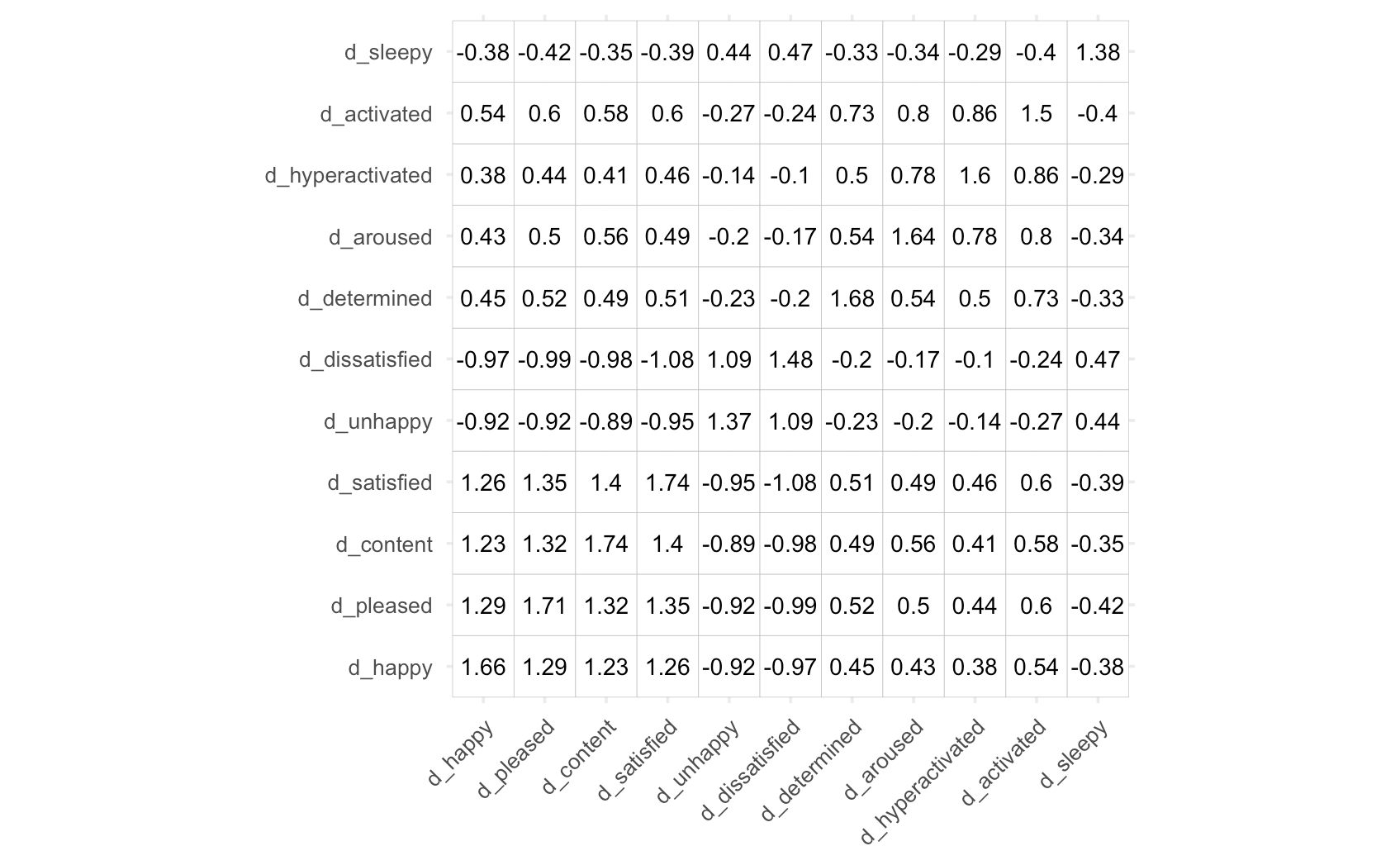
Covariance matrix from a study on human emotion

If we now plug in the formulas for PCA and EFA in the place of X, we get the following results.

PCA	FA
$$ R = \frac{1}{(n-1)}(Z_sD^{1/2}U')'(Z_sD^{1/2}U') \\ = (UD^{1/2})(UD^{1/2})' \\ =FF' \\ \approx F_cF'_c $$	$$ R = \frac{1}{(n-1)}(\Xi\Lambda'_m + \Delta)' (\Xi\Lambda'_m + \Delta) \\ =\Lambda\Lambda' + \Psi \\ \approx \Lambda_c\Lambda'_c + \Psi $$

Ignoring differences in notation $ F $ and $ \Lambda $ are functionally the same - there is quite some similarity. The subscript $ c $ serves to indicate that we reconstruct the covariance matrix using a lower rank approximation, using only the first $ c $ components or factors to reconstruct the covariance matrix. For the FA model, the added parameter $ \Psi $ serves to improve estimates of item-specific variances over what is possible in PCA. This explains why FA is said to reconstruct the shared variance (covariance), while PCA is said to explain the total variance.

Why is this a big deal?

Using the Eckart-Young theorem we can prove that PCA optimally reconstructs the totality of the covariance matrix. As an example, Iet's again look at the covariance matrix of the emotion items used before. I ran both PCA and FA, specifying a 2 component/factor solution. We can then reconstruct a lower rank matrix $ R_{rec} $ and subtract this new matrix from $ R $ to get a matrix of residuals, $ R_{res} $ :

$$ R_{res} = R - R_{rec}. $$

Taking the Frobenius norm $ \| R_{res} \|_F $, we get a good idea of how well the observed covariance matrix was reconstructed:

PCA	FA
$$ \| R_{res} \|_F^{PCA} = 2.3205 $$	$$ \| R_{res} \|_F^{FA} = 3.5561 $$

Indeed, we see that PCA offers a better rank $ 2 $ approximation of the covariance matrix. So why would we even bother with techniques that offer poorer performance?

Recall that for FA we are really only interested in the covariances. Rather than reproducing the whole covariance matrix, we care more about reproducing the off-diagonal elements of the covariance matrix. For this reconstruction, PCA is not necessarily the most optimal procedure. If we set all diagonal entries of $ R_{res} $ to zero and take the Frobenius norm of the resulting matrix, we get an estimate of the reproduction error for the off-diagonal elements. While PCA might optimally reconstruct the total covariance matrix, FA is better at estimating the off-diagonal elements of the covariance matrix.

PCA	FA
$$ \| R_{off} \|_F^{PCA} = 6.5712 $$	$$ \| R_{off} \|_F^{FA} = 5.9352 $$

Of course, all statistical procedures or models make some assumptions. Let's discuss what should be kept in mind when using PCA or factor analysis.

Assumptions

All observations should be complete, and significant outliers might bias the results. This is because both techniques, on some level, assume multivariate normality of the data. Let's go over some of the more substantial assumptions.

Both techniques also assume that the variables are correlated to at least some degree. If all variables were independent from one another we would not reach identifiable solutions for either PCA or FA. Since correlation is a linear measure of association, if the variables are only associated in nonlinear ways, the output of both models will be biased. Of course, both models are sufficiently robust against small deviations, especially when the variables are still monotonically associated. Solutions to deal with nonlinearity exist for both PCA and FA, but this is outside the scope of this blog.

Finally, a crucial difference between PCA and FA is that because PCA attempts to model the variance in the data, it is highly susceptible to differences in that variance. More concretely, if one variable has a variance of 1000, and the other variables only have a variance of 10, most of the variance lies in the first variable. As a result, the principal components will be dominated by the first variable. For this reason, it is always best to work with standardised variables. While this is not strictly necessary when doing factor analysis because it is scale invariant.

When and how do I use PCA or FA?

Say you want to apply either technique to help solve some problem you are having, which technique is appropriate?

PCA

PCA can be used as a dimensionality reduction technique assuming the assumptions discussed earlier are not violated. One important consideration is how many principal components to maintain. As a general rule, only components with an eigenvalue greater than one should be retained. This is because components with smaller eigenvalues don't explain additional variance over what could be explained using just one of the original features. This rule should generally give a very good indication of how many components to use. Should it be necessary, more numeric techniques like Horn's procedure exist that account for sampling variance in the eigenvalues.

Once the PCA has been fit, the components can be used as input to another model. This can be any kind of model: regression, classification, or even another unsupervised learning algorithm like cluster analysis.

FA

Factor analysis was developed to analyse data from questionnaires and to estimate the latent variables causing them. This was usually done to gain some more theoretical understanding of concepts being studied. As an example, psychologists has identified 5 dimensions of personality that can be consistently found across people of all ages and backgrounds. These dimensions were first identified using factor analysis. For these reasons, perhaps the most straightforward use of factor analysis within a business would be to analyse questionnaire data that has some latent structure, for example customer or employee satisfaction. With FA, questions that don't contribute much information can be identified and changed, or left out entirely.

To determine how many factors are to be extracted, the same methods used in PCA can be applied. However, in contrast to PCA the factor solution changes depending on how many factors were calculated by the model. More concretely, when calculating a 3 factor solution, the first 2 factors of that solution are not identical to the 2 factors of a 2 factor solution. As such, once it has been decided how many factors to use, it is best to recalculate the model and specifying exactly how many factors to retain.

To summarise, FA can be used to check whether a valid latent structure can be found, and whether or not the questions were interpreted similarly across different groups of people. Additionally, factor scores can be calculated and used as input to a machine learning model just like PCA. But, because FA is a more complex model (recall the extra parameter $ \Psi $ ), it should be preferred over PCA when the variables or features were measured with any degree of measurement error. A great illustration of this is given on the scikit-learn documentation for factor analysis.

However, a downside to FA is that because of this added complexity a solution isn't guaranteed to be found. This is both a blessing and a curse though, because when a solution cannot be found this usually means the model is very badly specified. At that point, you should turn back to the drawing board and rethink your model.

Conclusion

This blog introduced you to PCA and factor analysis by showing how similar the models are, but also highlighting crucial differences. Factor analysis and PCA have a lot in common, and are both a great first attempt at dimensionality reduction. As with all techniques, it is important to keep in mind which assumptions are made, and to choose the right tool for the job.

Keep posted for our next blog in the statistics saga, the interval between this blog and the next shouldn't be too large!

Acknowledgements

Thanks to Michelle Yik for allowing us to use the data from the valence/arousal study to serve as an example!

References

Yik, M., Mues, C., Sze, I. N. L., Kuppens, P., Tuerlinckx, F., De Roover, K., Kwok, F. H. C., Schwartz, S. H., … Russell, J. A. (in press). On the relationship between valence and arousal in samples across the globe. Emotion.