

By Giliam Rosseel, Liesbeth Bogaert, Yannou Ravoet, Chiel Mues
Anyone who has spent some time in Belgium/Flanders probably knows that road cycling is very popular around here. Competitions receive lots of media attention and almost every Sunday you will surely find a large group of amateur cyclists taking the road.
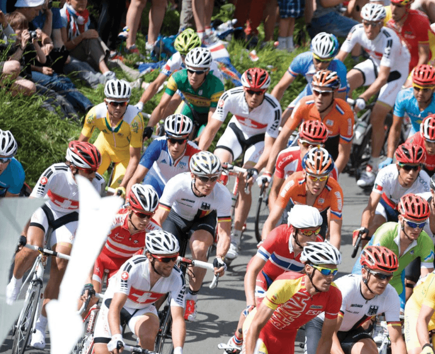
Figure 1: Typical Belgian Sunday [1]
A great source of discomfort or injury is an improperly adjusted saddle height [1]. Professional cyclists can fall back on their team for support and expertise. But this is not the case for the amateur cyclist, and a professional bike fitting can be quite costly, ranging between €200 and €300.
The process of perfectly fitting a bike to a person’s specifications and preferences can be difficult. Nevertheless, one quick fix that has substantial influence on a cyclist’s comfort is the saddle height. As described in Burt (2014): “Optimum saddle height is described by the natural position of the leg fully extended at the bottom dead centre (BDC) of the pedal stroke” (p. 41). Using AI we can detect the inner-knee angle and help cyclists adjust their saddles to the proper height.
Our low cost solution only requires the user to own a home-trainer and a smartphone or camera. All the user needs to do is upload a short video of themselves cycling the home-trainer. The video can be taken from any type of camera, and simply needs to be taken from a perpendicular side-perspective as shown in Figure 2.
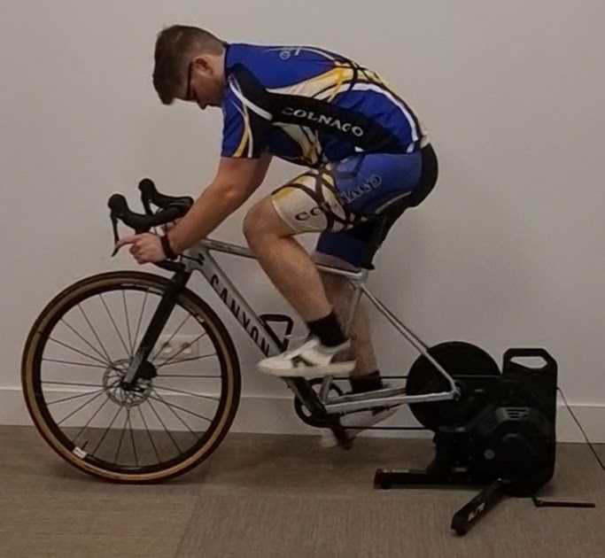
Figure 2: Example set-up
In this blogpost we present our easy-to-use application and the technology used to build and support it. What follows is an explanation of the model architecture we used followed by a step-by-step overview of how the video is processed and transformed into a recommendation. We discuss the robustness of our solution and explain how it is deployed and supported through Microsoft Azure, Terraform, and Github. Some technical details are provided - in the technical overview boxes - but these can be safely skipped by any reader.
Modelling
This section details the necessary steps to go from a raw video to the calculation of the knee angle and the return of a recommendation for the saddle height. First the core of the solution is introduced: the AI model (MoveNet); then the pre-processing and post-processing steps are described which lead to the knee angle calculation and the recommendation.
MoveNet
MoveNet is a lightweight pose detection model published by TensorFlow that can process images at real-time speeds [4]. This makes it perfect for estimating body keypoints in each frame of a video. The model finds 17 keypoints along the human body that map out a shape that is functionally accurate and sufficiently granular to distinguish the many different movements our body can make. Two versions of the model have been published: MoveNet Lightning and MoveNet Thunder. We use the more accurate, and still ultra-fast Thunder variant.
MoveNet architecture
The reason the MoveNet models are capable of faster than real-time inference is that they reduce the quality of the input image to a 256 by 256 pixels square (192 by 192 pixels for the Lightning model) [2].
The model is a combination of a feature extractor CNN that ends with 4 prediction heads: a Person center heatmap, a Keypoint regression field, a Person keypoint heatmap, and a 2D offset field per keypoint. The Person center heatmap can be used by the classifier to reject predictions of people in the background. The Keypoint regression field is used to find an initial set of keypoints. This set of keypoints can be used as a weight for each of the pixels in the Person keypoint heatmap. This ensures that keypoints from background bodies are not accepted. A final sub-pixel precision can be achieved by adding the 2D offset field to each keypoint. An overview of these four predictor heads is shown in the four pictures below. The complete architecture of the feature extractor combined with the predictor heads is found in the image below.
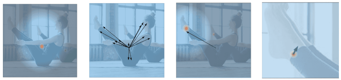
Figure 3: Visualization of the 4 prediction heads [3]
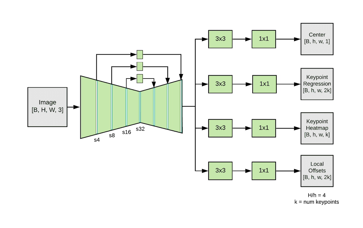
Figure 4: MoveNet architecture with B=batch-size, H=height, W=width, k=17 (# of keypoints) [3]
Pre-processing
Before the video is given to the MoveNet model some preprocessing needs to happen. Firstly the middle ten seconds of the video are extracted and the rest of the video is discarded. We do this because a person is more likely to be on their bike in the middle of the video versus in the beginning or end. Secondly, the resolution of the video is downscaled. Modern cameras and phones are very high in resolution. Unfortunately, this increase in image quality comes with an increase in file size. Larger file sizes greatly increase the model processing and the rates at which the video is up and downloaded. We downscale each video to be 256 pixels vertically, and auto-scale the horizontal dimension to preserve the aspect ratio. Thirdly, we reduce the number of frames per second in the video to 15. The reasoning is the same as before, more frames per second correspond to a larger file size, which increases processing time.
These limits were found to be the optimal tradeoff between accuracy and performance, reducing the time it takes to run the model without losing accuracy on the predicted keypoints. We discuss this in greater detail in the section on robustness.
As a last step, the video is converted into the proper format for the MoveNet model.
Cropping
We crop the input around the detected body to ensure that only useful pixels are passed to the model. This is done by creating a bounding box around the keypoints predicted in the previous frame and adding some extra space to allow for movements between two frames. The cropped image is a 256-pixel square as this is the input shape required by the MoveNet Thunder model [2].
Model Output
The model outputs a skeletal outline of 17 keypoints on the body, as shown in figure 5. More concretely, the model outputs the {y, x} coordinates of these 17 keypoints for each frame in the video. Remember that we are interested in the inner knee-angle, so we are not done yet. Post-processing of these keypoints is needed to get to a final recommendation.
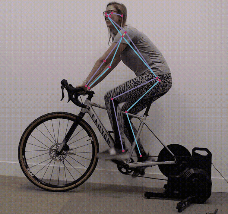
Figure 5: Skeletal mesh returned by MoveNet
Post-processing
Lowest Point
Due to the nature of the problem, we are really only interested in the knee-angle at the lowest point in the cycling motion. Plotting the y-coordinate of the ankle keypoint over time helps us to determine in which frame the pedal is at its lowest point.
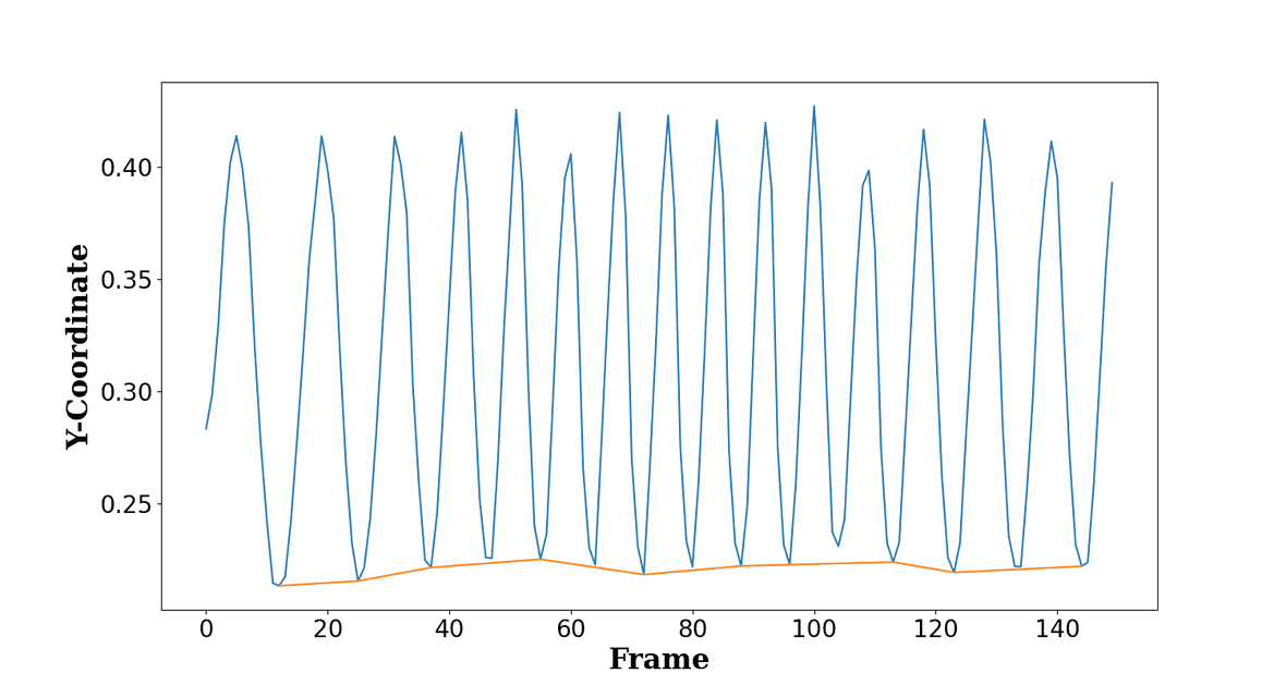
Figure 6: Y-coordinate of ankle keypoint for each frame
Lowest point calculation
To find the lowest pedal points, we look at the y-coordinate of the ankle that is facing the camera. We find the peaks of these y-coordinates by looking at local minima. To ensure that we only use the actual lowest points, we filter out some of the inaccuracies of the MoveNet model by adding the criterion that peaks should be separated by at least 10 frames; only the highest peaks within that distance are kept. More filtering on the lowest pedal points is done once the angles are calculated.
Knee Angle Calculation
Having identified the frames in which the ankle is at the lowest point we can now calculate the knee-angle. Only basic mathematics is needed to calculate the angle between three points.
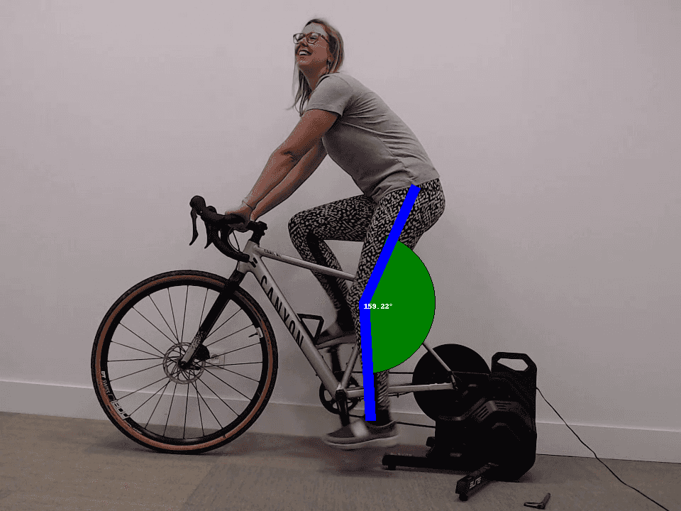
Figure 7: Example of a calculated knee angle
Knee angle calculation
Instead of calculating the angle between three points, we calculate the angle between two vectors. Where u is the vector starting at the knee and terminating at the thigh keypoint, and v is the vector starting at the knee and terminating at the ankle keypoint. The formula is given as a reference.

After calculating the knee angles at each of the lowest pedal points, we further filter bad predictions by removing any angle values below 130° or above 170°. We then perform one last filtering based on the distance of each predicted angle to the median of all predicted angles.
Recommendation
After processing, we end up with a distribution of angles at the identified lowest points. Angles that are at a large distance from the median are filtered out. However, any one angle might still contain some noise. For example, we cannot observe the position at the true lowest point because that point might lie in between two different frames. The mean of all the observed angles should be a good estimate of the angle at the true lowest point. We use this mean angle for our final recommendation.
Choosing a reference angle also requires some consideration. No perfect reference angle exists for any given situation or person. One might prefer performance over comfort, or vice versa. Based on Burt (2014) we settled on 145° as a reference angle for our recommendation. We chose this angle because it is a compromise between performance and comfort.
To introduce some tolerance, our recommendation assumes any angle between 140° and 150° degrees to be satisfactory. For angles that fall outside of this range, we give the recommendation to either increase or decrease the saddle height. Of course, if you want to continue adjusting your seat height to a specific angle you can continue using the predicted angle to fine-tune your bike configuration.
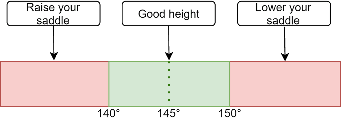
Figure 8: Range of accepted knee angles
Now that we have gone over the model and how it produces the results. An important question is how robust the results are to different specifications and user characteristics.
Robustness
The MoveNet models are trained on two labelled Datasets: a subset of the COCO 2017 keypoint Dataset containing 28k images with three or less people and the Active Dataset containing 23.5k single person images including images with motion blur and self-occlusions. The model performs similarly on people of different ages, gender or skin tones. Furthermore, the dataset contains people with different clothing, lighting and backgrounds [2].
Since we use the output of the model simply to calculate the angle between three keypoints using the cosine-rule, our output robustness is heavily dependent on the robustness of the MoveNet model. Errors caused by self-occlusion are also filtered since outliers are removed for the list of angles used to make a recommendation.
Robustness to video quality
To research the influence of the quality of the video on the robustness of the solution, we recorded predictions of our solution for different videos under multiple input quality configurations. For each video we varied the fps value, resolution, and duration. Specifically, the duration parameter is the number of seconds we use to find angles at the lowest pedal points. The fps and resolution parameters are simply a downsampling of the original quality of the input video.
For each configuration we record the values of the angle at the lowest pedal point. To measure the influence of a reduction in quality we look at the standard deviation of the angles. A higher standard deviation for a configuration means that the angles used to make the recommendation are more spread out and thus our recommendation is less precise.
To visualize the effect of a specific parameter on the robustness of our recommendation, we group the configurations by each of the parameters and look at the mean of the standard deviations across all videos. This is visualized in Figure 9 where the leftmost point on the fps plot shows the average standard deviation over all videos when reduced to 15 fps (regardless of resolution or duration). Overall, because outlier angle-values are filtered out, the standard deviations remain low, between 1.0 and 1.5.
Although decreasing the fps value of the video lowers the robustness slightly, the standard deviation is still low enough to make accurate recommendations. More frames per second means that the pedal will have moved less between frames, thus making the frames where the pedal is at its lowest point in the cycle, closer to the real lowest cycle point.
In terms of resolution we see that MoveNet is quite robust to low resolution images, with no discernible difference between the resolutions. We remind the reader that the input resolution for MoveNet is 256-by-256 pixels, meaning that it has been optimized around this value.
A less straightforward pattern is observed for duration. Where we would expect longer durations to have a lower standard deviation, we observe the opposite. We can think of two explanations for this. Firstly, since we always take the middle seconds of a clip, longer duration clips are more likely to contain frames where the cyclist is not perfectly seated. Secondly, a shorter video duration leaves us with fewer angles to estimate the standard deviation with. Since the standard deviation of 5 second clips is likely underestimated, we chose a duration of 10 seconds as a trade-off between robustness and performance.
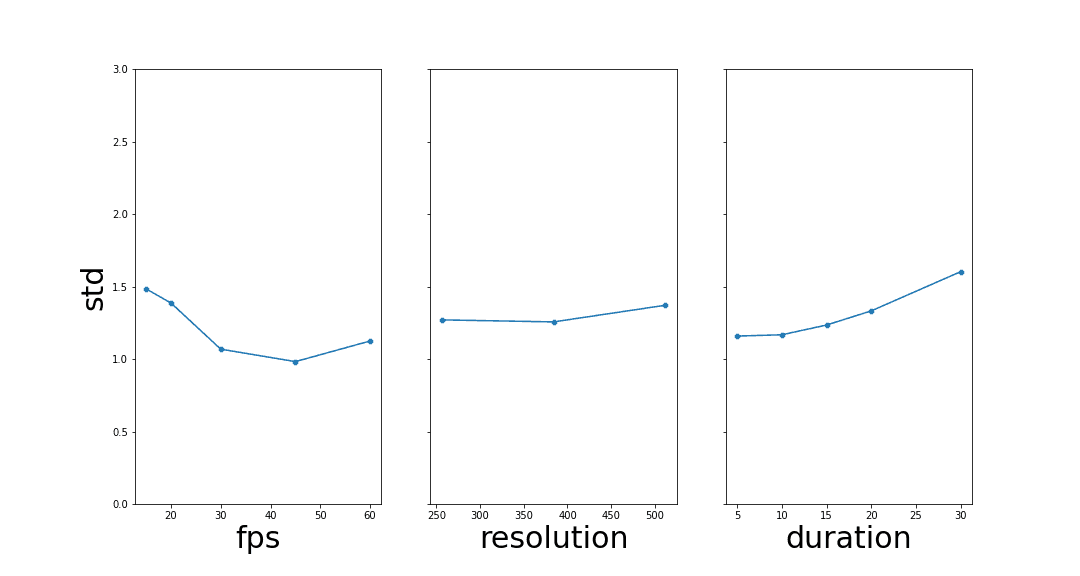
Figure 9: A study of the influence of input quality on recommendation confidence
Having explored the reliability of our solution we now discuss how it is deployed and supported by our chosen infrastructure.
Deployment on Azure
Our solution is hosted on Microsoft Azure. This platform was chosen because it is the biggest cloud platform in Belgium. To deploy our model and web service we split up the deployment into frontend, backend, and a function that connects them. The frontend is a Streamlit website deployed as an Azure App Service web app. This website serves as a user interface for uploading the video and displaying the results from the model. Computations of the model are all done on the backend. This backend consists of our ML-model pipeline, which is deployed as an API within an Azure ML Workspace.
To connect the frontend and backend, an Azure Function is triggered by a ‘blob event’ (storage trigger) whenever a new video is uploaded onto the web service. This function will notify the model that a new video has been uploaded, providing a path towards this new video. When the model receives this notification it will pull the video and start the machine learning process. When the model is finished the output will be stored in a results container. As this process is taking place, the website is continuously monitoring this container. Once the model output is available, it is immediately sent back to the website and visualised for the user.
The Blob storage that is used to link the Azure App Service and the Azure ML Workspace is immediately and automatically cleared once the data is used. Because we value privacy greatly, we do not retain any data - neither the uploaded data or the results - after the user has finished using our solution.
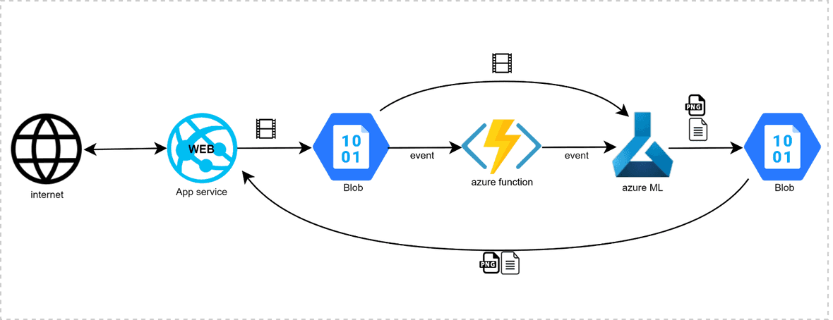
Figure 10: An overview of the infrastructure
Resources in detail
- Main Resource Group
- Storage Account: With ‘Videos’ container and ‘Results’ container
- App Service with Linux App service plan
- Azure Container Registry (ACR) with webhook
- ML Workspace with a key vault
- (Optional) Application Insights
- Function Resource Group
- Azure Function App with Linux App service plan
The Streamlit frontend is built as a Docker image and pushed to the Azure Container Registry (ACR). The Webhook that is linked to the ACR will notify the App Service when there is a new image available. The App Service deploys the docker image as a web app and makes it public.
The ML-model pipeline is registered and deployed in the Azure ML Workspace. This ML workspace creates a container instance for the model to run on; an endpoint is also created so that the model can be triggered by the Azure Function.
Two resource groups are needed because the service plans for the App Service and the Function app cannot share the same resource group.
CI/CD and IaC
While developing our application and infrastructure it became clear that recreating and organizing the necessary resources would become very difficult. An Infrastructure-as-Code solution would streamline this process. For deploying and maintaining infrastructure, Terraform supports all cloud-providers and services which makes it ideal for cloud-based applications. All resources needed to deploy our solution on Azure are described in our Terraform configuration files.
Our Terraform solution is supported by GitHub Actions and is set up as four GitHub workflows that continuously deploy new code as it becomes available.
GitHub Workflows
The first workflow is the frontend workflow. Its main job is building a Docker image of the frontend code and pushing it to the Azure Container Registry. The second workflow is the backend workflow. This workflow is responsible for running the python scripts which register and deploy the model pipeline to the Azure ML Workspace. After deployment, the model endpoint is returned. This endpoint needs to be specified in the Azure Function to enable the connection between the frontend and the backend. Both the frontend and backend workflows include linting and testing. The third workflow is responsible for redeploying the python code of the Azure Function when changes are made. The fourth workflow initialises, validates, plans, and applies the Terraform configuration files. By executing this workflow the resources described in the Terraform scripts are created in Azure.
Conclusion
We provide a low-cost and accurate solution that offers an easy-to-use alternative to the tedious and expensive bike fitting methods that are currently available. Using AI, we estimate the knee angles at the lowest points in the pedal cycle from an uploaded video. We use these angles to make a recommendation that optimizes the height of the user’s saddle. We open-sourced our code on github and provided easy-to-use deployment scripts so that anyone can replicate our solution.
Acknowledgements
We would like to thank everyone who helped make this project possible: the volunteers who helped create the cycling dataset, our colleagues at Dataroots who guided us through the project and the people of Tensorflow who made the MoveNet models publicly available.
Also watch our presentation of the project on Youtube!
References
[1] Burt, P. (2014). Bike Fit, Optimise your bike position for high performance and injury avoidance. London: Bloomsbury Publishing.
[2] Tensorflow (2021). MoveNet.SinglePose.
https://storage.googleapis.com/movenet/MoveNet.SinglePose%20Model%20Card.pdf
[3] Tensorflow (2021). Next-Generation Pose Detection with MoveNet and TensorFlow.js.
https://blog.tensorflow.org/2021/05/next-generation-pose-detection-with-movenet-and-tensorflowjs.html
[4] Martín Abadi, et al. (2015). TensorFlow: Large-scale machine learning on heterogeneous systems. Software available from tensorflow.org