Next best action recommendation - part 1: measuring the effect of a campaign

Campaigns you said? Great but which one? Multiple ways exist to nudge customers: for instance calling, sending out emails, offering discounts, etc. The channels are various and the content of the marketing messages are even more diverse.

In this article we explain how to optimize a marketing campaign and what to do when you did not implement the ideal strategy but have data that can help you derive important insights.

From churn prediction to business value

Not so long ago, in a previous post, we wrote about churn prediction.

Customer churn in the utilities sector - Silke Plessers

As the surge in gas and electricity prices intensifies with the UK and European gas prices even closing at ten times their level from the…

dataroots

We ranked customers from the ones with the highest risk of switching brands to the ones with the lowest risk. Of course, this is all quite neat, but there does not lie any business value in merely knowing which customers are at risk. We want to nudge these customers into staying, by targeting them with retention campaigns.

The holy grail for marketeers is to send the right message, through the right channel, at the right time. This involves discovering which of the customers at risk can still be persuaded to stay with the company and which are lost causes as it will be a waste of resources to target the latter. Sometimes, it even takes more than one marketing action to convince a customer while some other customers react in an adverse manner to the nudge. Optimizing a marketing campaign is an art to master.

In this post, we propose a methodology to optimize a marketing campaign and find out which actions (or which sequence of actions) will have the most beneficial impact on a particular customer.

There will be 2 other posts following this one, the next post will deep dive into causal inference, the techniques used and how they can be applied. The third post will deep dive into how to recommend an action and the reinforcement learning techniques that we used.

Let's start from the beginning: experimentation. Before drawing any conclusion, we need data in order to confirm or affirm our hypothesis.

The key is randomisation

The vocabulary that we will use in this post originates from the healthcare domain. Indeed, in this domain, a lot of experiments are made to evaluate the efficiency of new drugs, new treatments and their side effects. The treatment group is the group of patients treated with the new drug (in our case, the treatment is a marketing campaign / action).

Something we can learn from the healthcare world is that, when trying to evaluate the effect that a treatment will have, an experiment is initiated. They set up a target population, which should benefit from the treatment and then assign the treatment to only part of the population in a randomised way. That means that the treatment is given to the candidates at random. This allows to control for all the other factors that might also influence the desired outcome. Only then can you really assess whether the treatment is effective and whether some candidates respond better to it, and who these candidates are (i.e. what characterises them).

The need for a model

With a marketing campaign, the situation is not exactly the same. In a healthcare experiment, you try to solve a precise problem, such as to cure a certain decease. So you usually inject the treatment to already sick patients (target population) and evaluate the effect. In our case, you do not exactly know who the churners are and once a customer has churned, it is usually too late. Hence you need to predict who can be the churners. In this situation, a model can come in very handy.

Ideal marketing strategy

Once you have the model, a classical strategy is to choose customers with a high probability to respond well to the campaign. In our case, the target population would comprise of the customers who have a high propensity to churn. Similarly to the healthcare experiment, to be able to measure the effect of the campaign in an unbiased way, a random sample of the target population (high churn propensity) is set aside to control for the effect of the campaign. It is the best way to tell whether the campaign was successful and to measure the effect of the campaing (average treatment effect).

It is also common to select a random sample among the remaining population and include them in the campaign. This will serve the purpose of experimenting with other customers and possibly improve the way the target group is selected in the next iterations.

Eventually, we end up with 4 different groups (with H (L) being high (low) propensity to churn and T (NT) being targeted (not targeted) by a campaign):

With the above strategy, it is easy to measure the effect of an action: at the end of the campaign, you can just observe the average treatment effect as the difference in churn rate on the different groups. With a statistical test, we can even determine the significance and confidence interval of the treatment effect.

Reality check

In our particular case, the data available included information about the client (such as demographics, contract data etc.), information about the interaction between the client and supplier (such as complaints, emails, calls) and information about the campaigns (such as when a customer was targeted by which campaign and whether that customer belonged to the test or control group of that campaign).

Unfortunately, we did not have the luxury of knowing which purpose the marketing campaigns served or how the test and control group assignment was decided upon.

Consequently, we first needed to find out if these campaigns were indeed targeted at reducing churn and whether they had a positive impact on the churn rate.

Did the campaign have an effect?

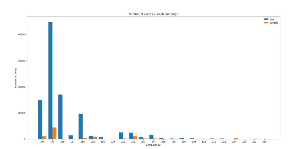
The first challenge we encountered was based on the fact that the size of the control groups already available in the dataset was much smaller relative to the treatment group size. This makes it more difficult to fairly evaluate the effectiveness of the campaign.

This problem can be solved by creating synthetic control groups. In a nutshell, the goal is to find a control group population with similar characteristics (similar feature distributions) as the treatment group population. This allows to eliminate bias and to control for other factors, and to evaluate the average treatment effect almost as if we had followed the ideal marketing strategy.

We tried out three different techniques to achieve this goal: we created synthetic control groups by applying the propensity scoring and coarsened exact matching (CEM) methods as well as using an ordinary least squares regression to estimate average treatment effects. The details on these techniques will be explained in the next blog post on causal inference!

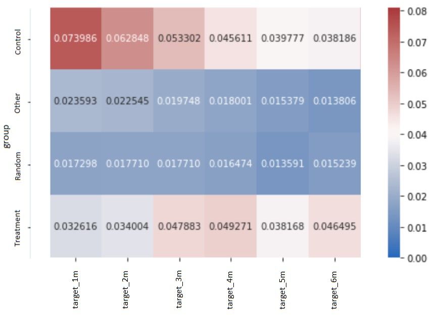
In the below image, you can see the different groups that were created with the synthetic control group method and their respective churn rate for each group, one month after the campaign (target_1m), two months after the campaign (target_2m), etc.

First, we observe that there is indeed a significant difference in churn rate between the treatment and control group. We can also see that this difference fades out after 2 months. Hence we could conclude that the campaign's effect lasts for 2 months. Secondly, also very interesting, the control and treatment groups have higher churn rates than the random and other groups. We can assume that the campaign was actually targeted at high churners and that it had the desired effect.

For other campaigns, it was more difficult to draw such neat conclusions.

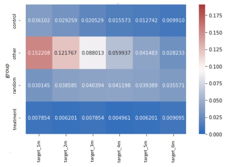
For example in the below campaign, it is the 'other' group which has the highest churn rate. Furthermore, even if there is a difference in churn rate between the treatment and control group, it is difficult to conclude that the campaign had the desired effect of reducing churn and was targeted at high propensity churners.

So the synthetic control groups help us conclude whether the campaign was effective on the treatment population.

Following a similar technique, we can even go one step further and instead of splitting the population in only 2 groups (random and treatment), we can have a more granular split which will allow a more thorough view on the effect the campaign had on different strata of the population. We will discuss this into detail in our next post.

Finally, since our ultimate goal is to improve the campaign targeting, we would also like to know whether we can recommend an action that will have more effect on a particular customer.

How to go from average treatment effect to recommending the perfect campaign?

We can start by learning a simple baseline logistic regression model. This model will be trained on the features and on the treatment variable (whether targeted by a campaign (and by which) or not) and will learn to predict the propensity to churn.

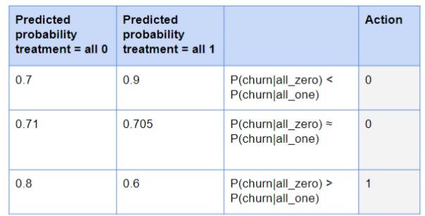
We use this logistic regression model to then predict the probabilities of churn on the test set whether targeted or not (treatment variable set to 0 and 1).

If the probability when treated is higher than when not treated, then do not target this customer with a campaign since you will waste resources on this customer as well as you will increase the risk of churn when targeting this customer (= lose-lose situation). Additionally, if the difference between the predicted probabilities is small, then also do not target the client with a campaign. Consequently, only target those customers where the predicted probability of churn is much higher if not treated with respect to if treated.

This approach shows promising results when only one campaign is considered but has trouble when it needs to differentiate between different campaign effects.

How to do better than this?

So now we have a baseline model. Unfortunately, there are still some drawbacks to just using a logistic regression model to recommend a new action. It can for instance not incorporate the future. With other words, it can only see if that client will churn that month, but not if he will churn the month after. Hence, if the action would have for instance a negative effect, but that effect would only be visible the month later, the model will not know this. Additionally, it cannot leverage the sequential nature of the data. We now have for each client for each month a record in the dataset. The logistic regression model cannot look at this sequence of data for each client to then decide when to take an action (if an action is necessary). The sequence of data however may harbor some interesting information regarding changing customer behavior that might be more difficult to capture by a logistic regression model. It hence can also not consider an optimal sequence of actions. It might be possible that for instance targeting customers first with campaign 1 to then target them again later on with campaign 2 will have the most positive effect on the churn probability. Finally, when being deployed, there is the additional disadvantage of the logistic regression model not being able to adapt to changing environment dynamics without retraining the algorithm.

Coming to the rescue is reinforcement learning! Reinforcement learning has many advantages over the traditional methods used to recommend actions. The specifics on reinforcement learning, its benefits, implementation and the results are discussed in part 3 of this series.

Remaining challenges

As previously mentioned, the first challenge we encountered was that we actually had no idea what the purpose of these campaigns were. We did not know if they were targeted at reducing churn or at some other goal. Furthermore, the control groups already available in the data were very small in size compared to their treatment groups and hence made it difficult to assess the campaigns’ effectiveness.

Additionally, the sparse and static nature of the data made it difficult to train a model. Very few features changed over time and the ones that did, were mainly sparse (such as complaints, emails, calls). This resulted in the features having a rather low predictive power which did not send a very strong signal to predict churn. This could partially be mitigated by performing some dimensionality reduction with PCA. Indeed, we found that the results after applying PCA on both the synthetic control groups as well as the reinforcement learning improved. By reducing the dimensionality and hence capturing most of the variance in the data by a lower number of features this problem was hence mitigated.

The final challenge was the highly imbalanced nature of the data. The data is skewed, often towards the non action consequence. We only have a small sample of the population that has been targeted and we do not know what is the reason nor what would have been the reaction of the other customers if they would have been targeted. On top of that, the target variable (churn) was also highly imbalanced.

Conclusion on the analysis

In this post, we went through the analysis of marketing campaigns and their effect on the churn rate.

We first described the ideal situation and strategy to create a marketing campaign that can be properly evaluated. Control and random groups were utilized in order to measure the effectiveness of the campaign and of the model used to identify the high propensity churners.

Since the data at our disposal was less than ideal - there was no information on the purpose of the campaigns nor was the control group size sufficient to assess treatment effect - we used synthetic control groups. This allowed to determine whether the campaigns had an effect and whether they were targeted at reducing churn. We will deep dive into this part in the second post of this series on causal inference.

As the ultimate goal of this analysis is to improve upon the marketing campaigns' effectiveness, we next went towards recommending campaigns. First we used simple logistic regression to recommend campaigns to certain customers. We then introduced the advantages of reinforcement learning over our baseline model. We will give a more in depth explanation on this in the third post of this series on reinforcement learning for next best action recommendation.

Finally, we exposed the remaining challenges that we encountered and we discussed mitigating actions we took and how the results could be improved.

Acknowledgements

Causal inference for The Brave and True has been a great guide during our analysis, and we would like to warmly thank the authors for compiling such informative and easy to read articles on causal inference.