Fine-tuning BERT for an unbalanced multi-class classification problem

1. Introduction

1.1 Context

As a Data Engineer at Dataroots, I was sent to a team in charge of promoting a Data Driven approach in the IT department of one of our clients. The major step was to set up a data lake to centralise the data from the whole IT department. One of the first use cases of this solution was to collect incidents occurring in the entire IT department, ranging from application crashes to server failures and service bugs.

With the huge amount of incidents generated on a daily basis, it was becoming difficult to manually track the allocation of each incident to a dedicated team. The information about each incident consists of only one row in a table with dozens of columns, such as incident number, severity, opening date, closing date and a description.

From there, we decided to create a Machine Learning model capable of predicting the team responsible for resolving an incident based on its description. The description column, being generally the most informative of all, was used to train the model. This required the use of Natural Language Processing (NLP) techniques to be able to use this column as input of the Machine Learning model.

1.2 Aim of this post

The aim of this post is to present the work that has been done for my client through the code that implements it, available in this notebook.

We'll be going through each part of it in order to detail not only the theoretical aspects behind each step, but also how to set it up in practice.

Despite the code that may seem complex at first glance, the tools available today make it possible to leverage the power of large models in a relatively simple way.

In fact, this exercise has been set up in an exploratory environment, i.e. with limited resources and time. Despite this, we were able to obtain satisfactory results which prove that this solution could be implemented in a larger context.

2. Methodology

2.1 The data

As part of this project, incident data was collected through a service management platform that provides companies with the ability to track, manage, and resolve issues. The data was extracted as a large CSV table, where each row represents an incident. Each incident is characterised by numerous columns that describe how it was logged, its priority, who it is assigned to, incident tracking, and communication about the incident between users,...

Unfortunately, as part of my job, I am not allowed to disclose any information from inside the company I work for. That's why in this blog post, I recreated an exercise with fake data but which reflects the real problem.

Here is an overview of what the data could look like.

2.2 The problem

Data quality is often compromised in real-world problems involving large amounts of data, and this can have a variety of causes. When an incident is recorded manually, there may be typos, errors or omissions in the information provided, or simply uncertainty about what information to fill in. For example, in this case, in a large organisation with hundreds of teams, it can be difficult to determine who to assign an incident to. On the other hand, when an incident is logged automatically, the information is usually very thorough, but it often lacks context. The script that generates this information provides only general information, which can make it difficult to understand the specific circumstances surrounding the incident.

When trying to determine the team responsible for an incident, it is essential to collect detailed information about the problem in order to be able to deduce the cause. Information related only to the incident ticket is not sufficient and does not allow a complete analysis. Therefore, it is more interesting to focus on the columns that precisely describe the context in which the incident occurred, the factors that contributed to its occurrence, as well as the possible interactions with other elements of the system.

One way to do this is to focus on the "description" column. This column is almost always filled in and contains information that describes the incident, whether it was filled in manually or generated by a script. Of course, other columns could also be relevant, but to simplify the process and since we have to start somewhere, limiting ourselves to the column that seems most relevant is a wise approach.

2.3 The solution

Now that we have a defined problem, we have to choose a way to solve it. This project, consists in using natural language processing (NLP) techniques to transform our data from language to numerical data and to be able to leverage the power of a machine learning model. To do this, different NLP methods were examined to encode the language and it was decided to use embeddings. In particular, the BERT model was used because it is considered the best model and has many advantages.

BERT is a deep learning based natural language processing model that is capable of capturing complex semantic information using multi-headed attention and bidirectional training. BERT is also capable of being fine-tuned for specific natural language processing tasks. Thus, by using BERT to solve a text classification problem within the company in question, it will be possible to learn the company's specific jargon. For example, if the company uses specific technical terms or acronyms, the model can be trained to understand and use these terms in its predictions. This can help improve the accuracy of the model by using data that is more relevant to the business.

More specifically, in our case we will use the bert_uncased version in its classification version. It has a specific classification architecture that will allows us to directly fine-tune the model for a multi-class problem.

3. Preprocessing

3.1 Preprocess the data

First of all, it is important to know that BERT incorporates pre-processing methods that are used automatically. Moreover, although these are powerful, taking the time to clean and prepare the data in a context-specific way can be really beneficial. That's why I took the time to clean the data myself beforehand. I consider that some words can be changed or removed without harming the important information, as they could be perceived as noise rather than meaningful data by the model.

In any case, data cleaning is a crucial step in the training process of any natural language processing model. It ensures that the input data is consistent and of high quality, which can greatly improve the accuracy and performance of the model. In addition, data cleaning can help reduce the risk of bias or error in model predictions by removing unnecessary or unwanted data.

3.1.1 Stop words

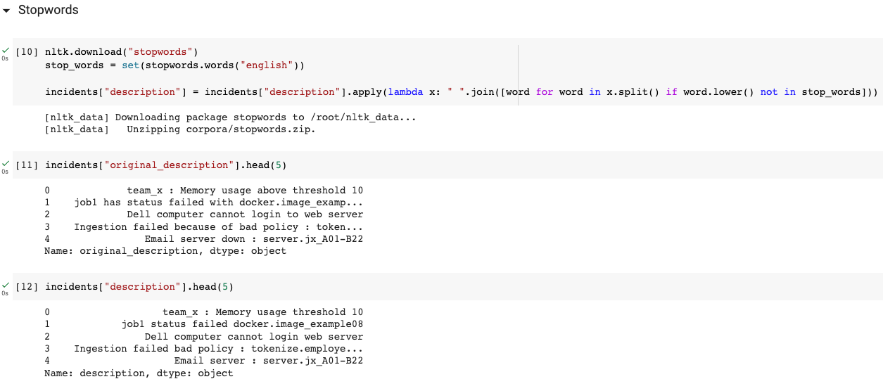
This first step consists of removing commonly used words in a language (such as the, a, an, and, of, ...) that do not carry a particular meaning or are not relevant to the specific context of the text analysis. This step reduces the size of the data and improves the performance of text processing models by eliminating background noise.

The NLTK library provides a corpus of "stop words" easily accessible online to perform this preprocessing step. It is also possible to remove some words from this list in case you don't want it to be considered as a stop word. Indeed, it is important to note that removing some words can alter the meaning of the text, so you must select the words to be removed with care.

3.1.2 Punctuation

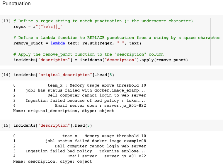
This step consists of simplifying the text data by removing punctuation symbols that do not carry useful information for text analysis. However, it is important to note that punctuation may have important meaning in some cases, such as in the case of sentiment analysis or dialogue, and can therefore be retained if necessary.

In our case, where the description is often short and unstructured, the formulation of the sentences is not very important and removing punctuation is appropriate. Secondly, it is common to find system or variable names in our data that are often strings of relevant words grouped by dots, commas or even underscores (e.g. docker.image_example08). Therefore, rather than simply removing punctuation, we will replace it with spaces and include underscores to be a punctuation character. This allows us to keep the information contained in these fields while avoiding increasing the complexity.

3.1.3 Lowercase

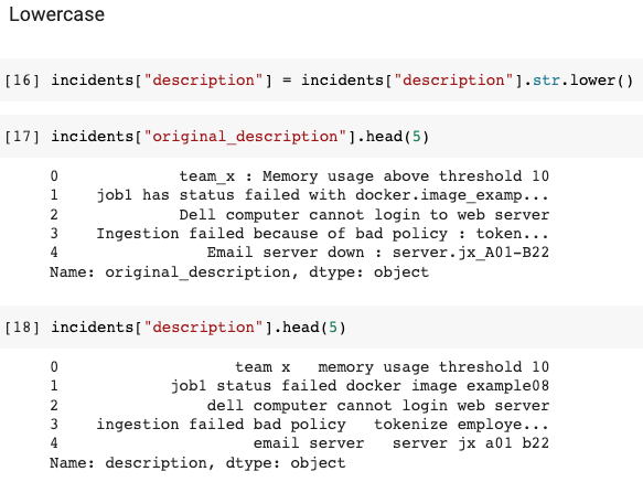
In retrospect I realised that this model is in fact "uncased". In other words, it makes no distinction between upper and lower case letters. This makes this step useless but I'll leave it, as it's still one of the most common pre-processing steps.

This step consists of transforming all letters into lowercase. It allows to normalise the text and to reduce the processing complexity for the models. Indeed, without this step, the models would have to process the same words in different forms (for example, "Hello", "hello" and "HELLO" would be considered as three different words).

3.1.4 Numbers

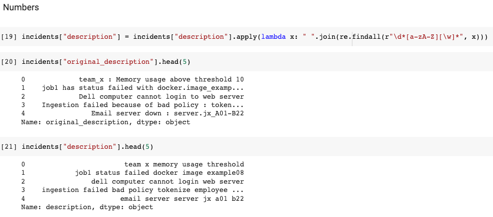
This step consists of removing all pure numbers (i.e. numbers that are not associated with letters) and reduces the dimensionality of the data by eliminating numeric characters that are not relevant for text analysis such as years, dates, phone numbers, etc.

3.2 Preprocess the labels

After preprocessing the input data, the next step is to preprocess the labels. These play a crucial role in multi-label classification tasks, as they represent the target variables that we want that our model predict.

3.2.1 Label distribution

A first important factor to consider in preprocessing labels is the occurrence of the different labels. Often, the labels can be highly unbalanced, meaning that some labels appear much more frequently than others. This can cause problems for the model to learn, as rare labels may not have enough data for the model to find meaningful patterns.

A second factor is the complexity of the problem. When dealing with a large number of labels, the computational complexity of the model can increase significantly.

Since this project is only a Proof of Concept, it is not necessary to solve these problems the hard way. What I will do is to limit the number of labels by grouping the less frequent labels in an other label. This way, I accumulate the occurrences of rare labels and reduce the complexity of the calculations.

3.2.2 Team occurences

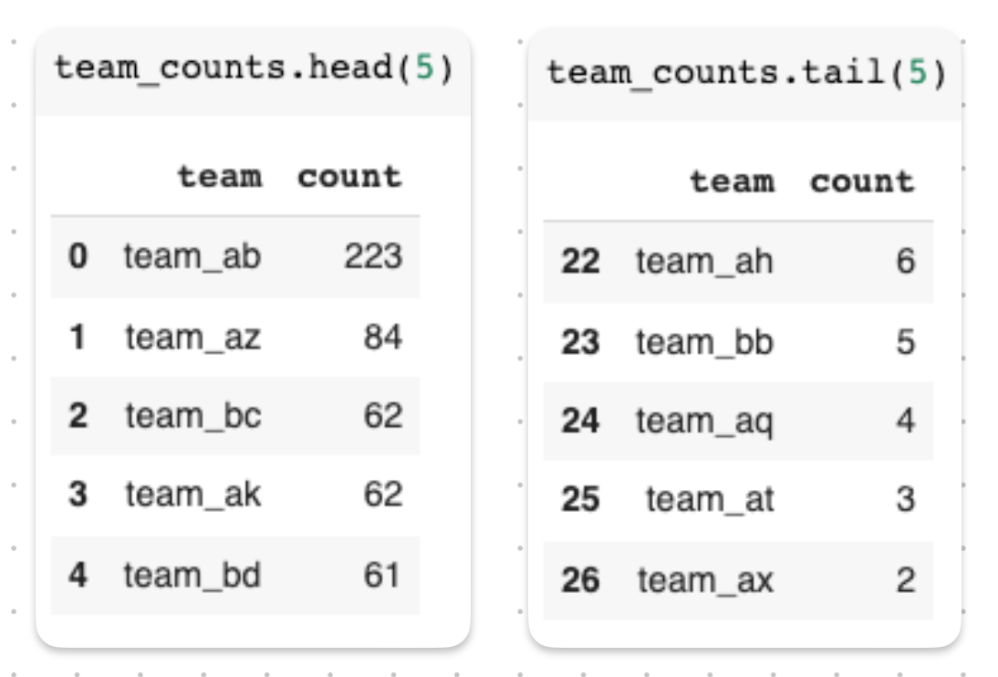
With the following code, we see that all our incidents are assigned to a total of 27 different teams and that they are indeed unbalanced

3.2.3 Team occurences above a quantile

In order to limit the number of teams taken into account I will use a quantile separation (which is totally arbitrary, but very practical)

In statistics, a quantile is a value that divides a data set into equal parts (e.g. the median is a quantile that divides a data set into two equal parts). The quantile 0.90 means that 90% of the values in the data set are less than or equal to this value, and 10% of the values are greater than this value. Therefore, in our example, the 0.90 quantile gives the number of incidents that has to be associated to a team such that 90% of the teams have fewer incidents associated with it.

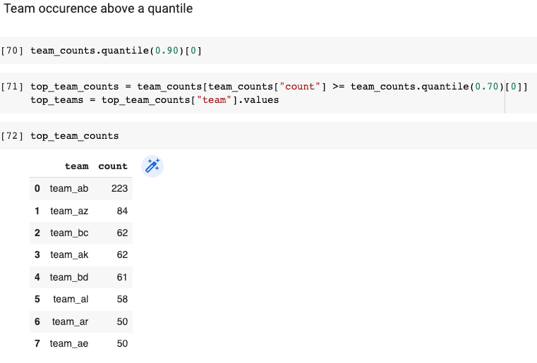
By taking the 0.70 quantile we are able to limit the number of teams to 8.

3.2.4 Match each team to a label

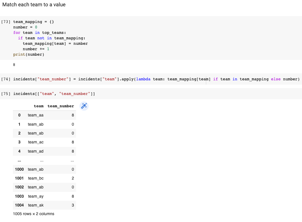
Now, rather than using the team names as a target, we will encode them with a label. By the way, all the teams that were not selected by the the quantile selection, will all be grouped together with the same label.

3.2.5 Team distribution plot

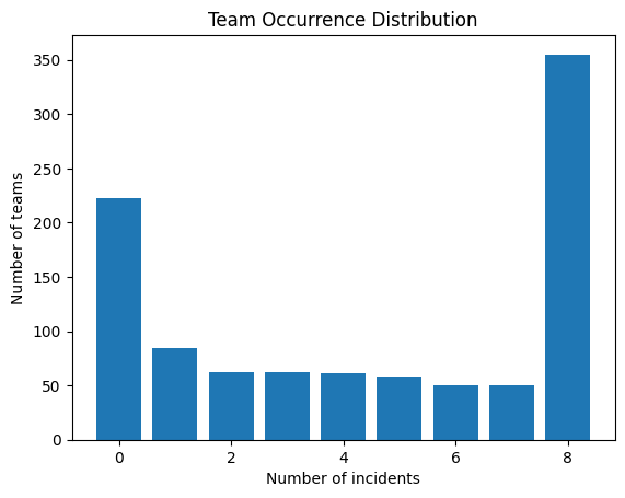
This step is twofold. It helps to reduce complexity by limiting unbalancness and it also helps to get a better idea of how our dataset is composed. However, even after that we can see that the effect is still there. This will be further fixed afterwards.

3.3 Split the data

Now the data has been prepared, it is necessary to do a first split of the dataset into two distinct subsets: the training set and the test set. This separation is essential to evaluate the performance of a machine learning model and to prevent overfitting.

Fortunately, the sklearn library provides a function called train_test_split() that allows for easy and efficient splitting of the dataset. The following code snippet demonstrates how to use this function to split the dataset into training and testing sets

3.4 Balance the trainig set

As mentioned earlier, achieving optimal training performance may require further balancing of the training dataset. To do so, the number of incidents in the training dataset is adjusted by equalising the number of incidents associated with each team. More precisely, we will take as a reference the number of incidents of the team with the fewest.

4. The model

4.1 Tokenization

Okay ! Now, the data has undergone our specific transformation but to use the BERT model effectively, the source will also go through the BertTokenizer library. This integrated tokenizer performs several steps of preprocessing to transform the input text into a BERT sepcific format :

1. Each input sentence is splitted into word-level tokens and mapped to their respective IDs in the BERT vocabulary.
2. Special tokens are added to mark the beginning ([CLS]) and end ([SEP]) of each sentence, with IDs of 101 and 102, respectively.
3. Sentences are padded or truncated to a maximum length of 512 tokens, with padding tokens ([PAD]) assigned an ID of 0.
4. An attention mask is created to indicate which tokens should be given weight by the model during training, with padding tokens assigned a value of 0.

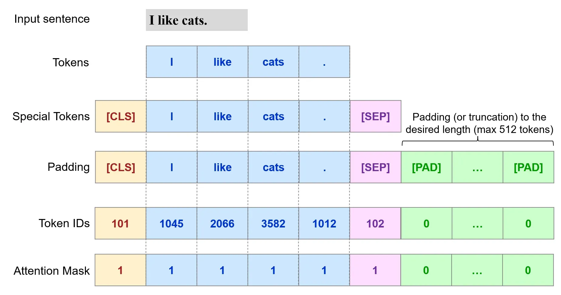
To perform these steps, we can use the tokenizer.encode_plus() method, which returns a BatchEncoding object with the following fields:

• input_ids : a list of token IDs.
• token_type_ids : a list of token type IDs.
• attention_mask : a list of binary values indicating which tokens should be considered by the model during training.

4.2 Split the data (again)

Now that all the data that will be used by the model respects the required format, it is necessary to split the dataset a second time. Indeed, this time, it is the training set which will be itself split in 2 datasets, the real training set (80%) and the validation set (20%).

In this case, the validation set is used during the fine-tuning of the BERT classification model to evaluate its performance and make decisions regarding hyper-parameter tuning. It helps in monitoring the model's progress, detecting overfitting, and optimising its configuration for better generalisation to unseen data. This is not to confuse with the previously made test set which is reserved for the final evaluation of the model

Note that, the datasets are encapsulated within a DataLoader PyTorch object, which simplifies their handling. By utilising a DataLoader, the datasets become iterable, allowing easy access to the data. This abstraction provides a more intuitive syntax for working with the dataset, enhancing the efficiency and usability of the code.

4.3 Training initialisation

Before we can start the training, some final specifications need to be set up.

First a few metrics are implemented to fit to our multiclass problem.

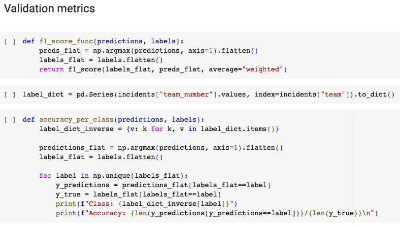
Then, the optimizer is created by providing it an iterable containing the parameters to optimize, along with specific options such as learning rate and epsilon (values chosen based on recommendations from the BERT paper). Finally, a learning rate schedule is instantiated. Its effect is to decreases linearly the learning rate from the initial value to 0. Also in the optimizer, you could have set a warmup period beforehand during which increases linearly the learning rate from 0 to the initial value in a specific amount of steps.

4.4 Training phase

The fine-tuning phase like it is build in the code given below, consists of two main parts: a training loop and an evaluation function.

The training loop iterates over multiple epochs, updating the model's parameters using batches of training data. It computes the loss, back-propagates the gradients, and updates the model's parameters. It also saves the model's state at the end of each epoch.

The evaluation function assesses the model's performance on a validation dataset. It calculates the average validation loss and obtains predicted logits and true labels for analysis. The function operates in evaluation mode to prevent parameter updates.

By combining the training loop and evaluation function, you can train the model iteratively, refining its performance over epochs and evaluating its generalisation on unseen data.

Let's see how these 2 steps work without going into too much detail but at least give you an overview of how the training works

4.4.1 The evaluation function

Let's first have a look at the evaluation function.

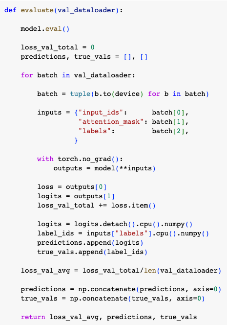
The evaluate function takes a DataLoader object as argument that will pass the validation data in batches. It first starts by setting the model to evaluation mode using model.eval() that ensures the model's parameters not to be updated during evaluation.

Next, it initialises variables loss_val_total, predictions, and true_vals to store the total validation loss, predicted logits, and true labels, respectively.

The function then enters a loop over the batches from val_dataloader. Within each iteration, the batch is moved to the appropriate device (e.g., GPU) using to(device). The inputs to the model are specified using a dictionary which contains the input IDs, attention masks, and labels.

Inside the with torch.no_grad() block, the inputs are given to the model as keyword arguments. The resulting outputs contain the loss and logits. The loss is accumulated in loss_val_total while the logits and labels are detached from the computational graph, moved to the CPU, and appended to predictions and true_vals, respectively.

After processing all the batches, the average validation loss is computed by dividing loss_val_total by the number of batches contained by val_dataloader. The predictions and true_vals lists are reshaped along the first axis using np.concatenate to obtain single arrays.

Finally, the function ends up by returning the average validation loss, the predictions, and the true labels.

4.4.2 The training loop

Now that you fully understand what happens when the function is evaluated, let's take a step back and look at the context in which it is used, namely the training loop.

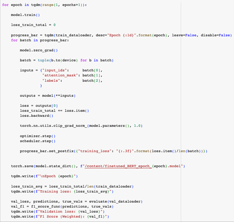
This loop iterates over the specified number of epochs. Within each epoch, the model is set to training mode using model.train() and a variable is initialized to store the total training loss.

A progress bar  is created using the tqdm library to visualize the iterations over the train_dataloader which provides the training data in batches. Inside each iteration, the model's gradients are reset using model.zero_grad().

Then, similar to the evaluate function, the batch is moved to the device, the inputs are wrapped in an inputs dictionary and given to the model through keyword arguments. The resulting outputs contain the loss that is accumulated in loss_train_total while the gradients are computed by calling loss.backward().

After that, a nice thing that is done is to limit the norm of the the gradient to 1.0 with the clip_grad_norm_() function to prevent them to explode.

Finally, the optimizer is updated with optimizer.step(),  the learning rate scheduler is stepped forward with scheduler.step() and the progress bar's is updated to display the current training loss.

After completing all the training batches within an epoch, the model state dictionary is saved and the evaluate function is called to display the validation loss and the F1 score.

4.5 The Prediction

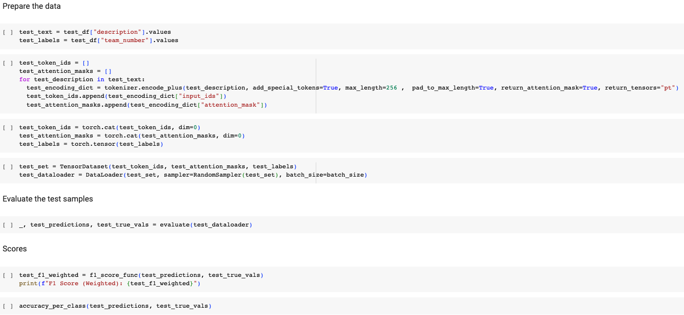
After a training procedure, we are finally able to assess the performances of the model on a test set that has never been seen by the model. To do so, we simply predict the class after having the the same data preparation as for the training. More specifically, the full tokenisation but also the wrapping, first in a TensorDataset and then in a DataLoader, is done. The evaluation, strictly speaking, is done with the evaluate function detailed above and we calculate the F1 score and the accuracy with the two functions you know.

4.6 The Embeddings

An important feature of the BERT model is that you can retrieve the meaningful embedding that captures the contextual representation of the input text which is here the whole description.

The only thing you have to do is to tokenise a sample the same way as in the training and prediction. Then, by passing the sample_token_ids and the sample_attention_mask to the model, it will produce various outputs, including the hidden_states. These hidden states represent the contextualised representations of each token at different layers of the model.

In the code, we retrieve the final hidden state, denoted by output.hidden_states[-1] which captures the most comprehensive contextual representation.

To obtain a single embedding for the entire text, we calculate the mean of the hidden states along the sequence length (dim=1). This mean pooling operation summarises the information from all the tokens into a single fixed-length vector, which represents the contextual embedding of the input text.

These embeddings can then be further used for various downstream tasks such as text classification, information retrieval, or similarity comparison.

5. The Results

Since the example code provided for this blog post uses random data, it would be impossible for any model to learn meaningful patterns. Therefore, the results that I'm about to present here are the ones obtained in the real exercise. In that case, I used a sample of 100,000 incidents out of the complete dataset, involving over 400 teams. Note then that, in the team filtering process, a quantile of 95 was used to limit the analysis to 10 specific teams and one "other" group. After balancing the data, I ended up with a complete sample dataset (train + validation + test) with a bit less than 1,000 incidents per team.

5.1 The Interpretations

The accuracy values for each team in both the validation and test sets are presented in the table below. It showcases the performance of the model in classifying incidents into the respective teams.

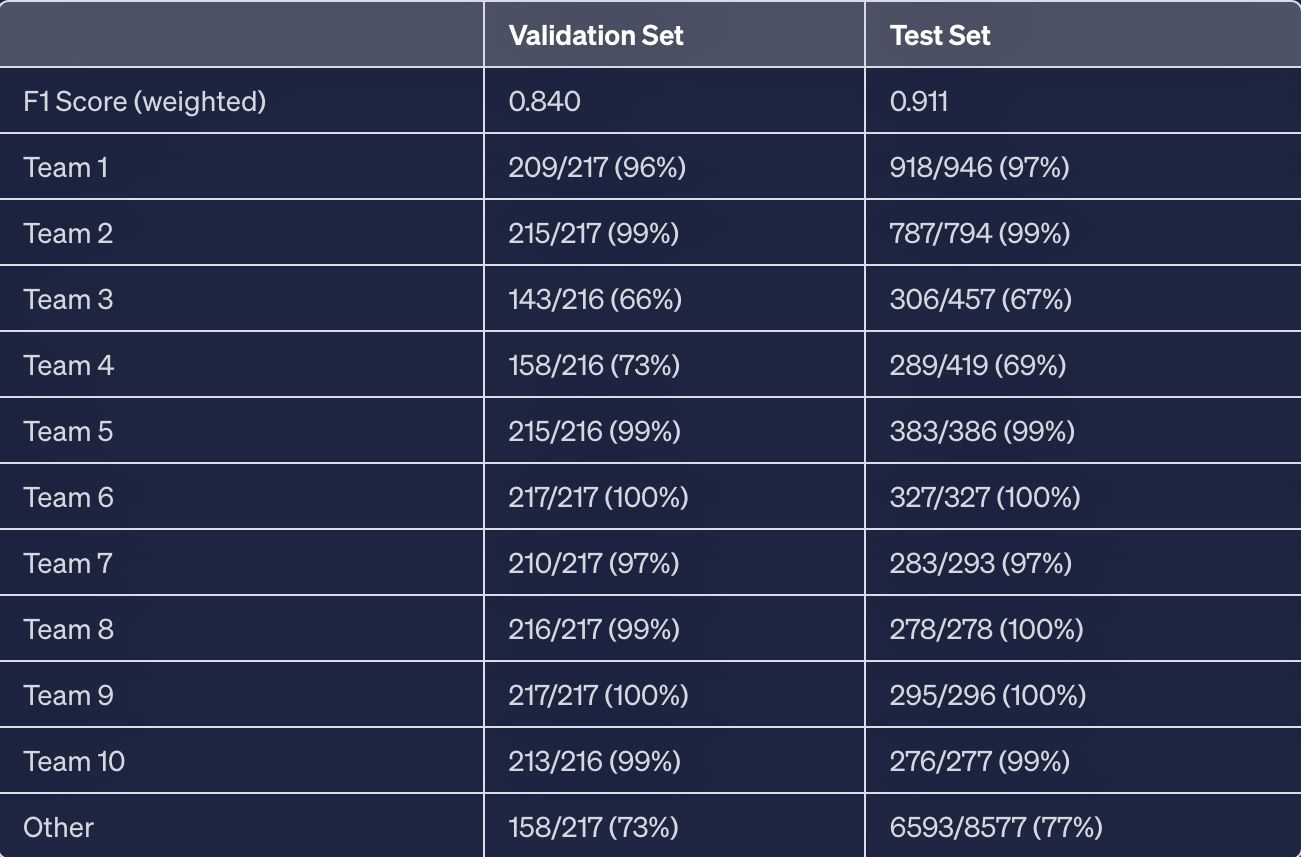
The obtained accuracy and F1 score metrics demonstrate that the model performs well in terms of precision, recall, and accuracy across all classes, taking into account class imbalances. However, some classes may pose challenges for the model, resulting in relatively lower accuracies.

I would like to emphasize the limited amount of data in our training set available for such a neural network. The model we are using, specifically BERT base uncased, consists of 12 layers, 768 hidden units and 12 heads, resulting in a total of 110 million parameters. The effectiveness of this model in our case is attributed to transfer learning. Through fine-tuning BERT, we are able to leverage the knowledge gained during its initial training, done on a large dataset called BookCorpus, which comprises 11,038 unpublished books and the entire English Wikipedia. By tailoring these acquired capabilities to our specific problem, we can achieve excellent performance.

5.2 The Discussion

5.2.1 The Limitations and Biases

The first thing that we see is that there are varying accuracies among different teams. This effect can be attributed to intrinsic factors in their descriptions. For instance, some teams may primarily use automatically generated descriptions that have a consistent structure, making them easier to differentiate. Additionally, frequently assigned teams might have more general descriptions, resulting in less specificity. It is important to note that specific explanations for these discrepancies are unique to the internal data and cannot be disclosed here.

Then, although its accuracy is quite good, the "other" group is not expected to have really high accuracy since it encompasses all the remaining teams. Its only specificity is not to be part of the 10 specific teams.

Finally, note also that, the F1 score is higher in the test set. This is logical since this dataset has not been balanced and therefore has a larger amount of the "other" incidents. That said, the F1 score should not be significantly influenced by the distribution of the teams.

5.2.2 The possible improvements

Although, as we've seen, this exercise had certain limitations, it demonstrates the feasibility of the task. Further improvements could involve utilising additional incident features (even other text features that could also be transformed into a specific vector) or employing data augmentation techniques to enhance model accuracy.

Also, the data quality used in this exercise is suboptimal. Nevertheless, NLP techniques manage to leverage the available free-text data, even if it lacks rigor or consistency.

And last but not least, the first area for improvement is certainly the number of incidents that this project covers. Indeed, in the real PoC, by limiting myself to 10 specific teams, I only cover a very small percentage of the incidents that occur, which makes the project quite useless... That said, given the good results, I am confident that this project can be developed further to cover almost all teams. Even if it means using this model more as an advisor rather than giving it the right to define an assigned team directly. In fact, this is what has been done! A similar model, rather than returning a single team, displays the top 10 teams with their associated probabilities to help a human to assign an incident to.

6. Conclusion

In conclusion, this blog post has shown us some important points. Firstly, we discovered that we can solve complex tasks quite easily by using large pre-trained models available in open source. These models provide us with powerful tools to tackle challenging problems effectively.

Despite facing limitations in time and computing power, we were able to demonstrate the feasibility of our initial problem by working on a simplified version (PoC). I have shared both the reflexion behind this simplified approach and the complete code that was used, allowing you to understand and explore the topic further.

By gaining insights into how BERT works and how to use it, you now have a solid foundation for future projects in the field of natural language processing. I hope this post has provided you with valuable knowledge and resources to begin your own similar works successfully.

Thank you for reading !

Antoine

7. Acknowledgement

I'm grateful to my colleagues who helped me with this project and shared their knowledge, which greatly influenced the content of this article.

I would also like to thank Dataroots and my client for allowing me to write about a subject internal to their company. This allows me to share my ideas with a wider audience.

I also want to acknowledge the inspiration I gained from the work of Nicolo Cosimo and Susan Li. Their excellent blog posts on a similar subject inspired and influenced my own writing.

Fine-Tuning BERT for Text Classification

A step-by-step tutorial in Python

Towards Data ScienceNicolo Cosimo Albanese

Multi Class Text Classification With Deep Learning Using BERT

Natural Language Processing, NLP, Hugging Face

Towards Data ScienceSusan Li

I also want to mention that I used ChatGPT, to help me write this blog post. While it improved my efficiency, it's important to remember to review and validate the AI-generated content for accuracy.

Lastly, I have made the entire code for this blog post available in my notebook. This allows readers to explore and replicate the findings discussed here.