Tracking Carbon Emission During MLOps

Machine learning (ML) models are becoming more advanced, allowing them to achieve impressive results across a wide range of tasks. However, this increased sophistication comes with a cost: ML models can be extremely computationally intensive to train. In recent years, the energy consumption associated with ML training has grown exponentially, and this trend is expected to continue. For instance, the training of the GPT-3 language model consumed 4.6 million kilowatt-hours (kWh) of electricity, which is equivalent to the annual electricity consumption of 500 American households¹.

Data centers, where the bulk of ML model training takes place, account for a significant and growing portion of worldwide electricity usage. According to the International Energy Agency, the estimated global data center electricity consumption in 2022 was around 340 TWh, which is around 1-1,3% of global electricity demand². By 2030, some estimates put this number as high as 13%!³ Despite advancements in cloud infrastructure and claims of efficiency, the energy-intensive nature of machine learning models remains a pressing concern, contributing to the escalating climate crisis.

The impact on greenhouse gas emissions from data centers and the energy-intensive nature of ML model training are issues that demand our attention and proactive solutions. In this context, efforts to quantify and understand carbon emissions play a crucial role. It enables us to grasp the true environmental cost of our AI and ML endeavours, helping us make informed decisions towards a more sustainable future.

Quantifying emissions using CodeCarbon

Embarking on the journey to reduce our greenhouse gas emissions begins with understanding our current carbon footprint. The CodeCarbon package emerges as a valuable tool in this endeavour.

Developed by experts from BCG’s GAMMA team, AI research institute MILA and Haverford College. The purpose of this tool is to enable ML engineers to track and better understand the carbon emissions generated during the development of their algorithms.

CodeCarbon calculates carbon dioxide (CO₂) emissions as a product of two factors:

CO₂ = Carbon intensity of electricity*Electricity consumed by infrastructure

The carbon intensity of the electricity is determined by taking a weighted average of emissions originating from various energy sources, such as fossil fuels and renewable resources, that contribute to electricity generation. This calculation produces a consistent value derived from data over multiple years, evaluated individually for each country. If the code is ran on the cloud, CodeCarbon utilizes the carbon intensity data of the country where the datacenter is located. Google Cloud stands out as the sole prominent cloud service provider that reveals the grid carbon intensity of its individual data centers. This enables us to employ the specific constant associated with the utilized data center rather than its geographical location. The second factor, energy consumed, is determined by tracking the amount of energy used by the infrastructure from both private on-premises datacenters and major cloud providers. If the code is ran on a local machine, energy is tracked of the RAM, CPU and GPU.

Although the CodeCarbon package offers valuable insights into carbon emissions, the current format of presenting the metrics as a standalone CSV file or dashboard can limit its adoption and integration into development workflows. To enhance the usability of CodeCarbon, Dataroots has developed the "MLFlow-emissions-sdk" package. The package seamlessly integrates the CodeCarbon package into the MLFlow MLOps package. Extending the logging capabilities of the widely-used MLFlow package with the carbon tracking methodology of the former.

mlflow-emissions-sdk: Integrating CodeCarbon into MLFlow

The package is open source and can be found on Github. In this section we will briefly go over how to install the package and give an example on how to use it.

How to install

First step is to install the package using pip. As a prerequisite, you need to have CodeCarbon and MLFlow separately installed for the package to run.

pip install mlflow-emissions-sdk

How to use

To make use of the package, you need to import "EmissionsTrackerMlflow" into your notebook or python script:

from mlflow_emissions_sdk.experiment_tracking_training import EmissionsTrackerMlflow

The imported class contains a number of useful methods for logging carbon related emissions metrics. Currently, the package supports PyTorch, Keras and Sklearn models. Prior to utilizing the package, you simply need to establish an endpoint for logging purposes. This can be achieved through an MLflow UI running in the background or an MLflow instance deployed on Azure ML or Databricks.

You can run MLFlow locally via:

mlflow ui

If MLFlow is running locally on your machine, then the tracking uri would be “http://127.0.0.1:5000”. In most cases, the model will be training on a cloud environment. For example Azure ML provides users with an MLFlow tracking URI:

Once you know the tracking URI of your MLFlow instance, you can then create a dictionary containing the:

tracking_uri
experiment_name
run_name
flavor (Keras, PyTorch or Sklearn)

Giving the following result:

tracker_info = {
    "tracking_uri": "<http://127.0.0.1:5000>",
    "experiment_name": "keras_test",
    "run_name": "keras_run",
    "flavor": "keras"
}

Once that is done, you can now instantiate your EmissionsTrackerMlflow:

runner = EmissionsTrackerMlflow()

The runner requires the dictionary defined earlier to create the proper MLflow’ context:

runner.read_params(tracker_info)

Running the function above will refer to the experiment with the given experiment name, if no experiment with the given name exists, then it will create an experiment. It will then also create a run with the given name. The flavor key is needed to make sure that your model is logged properly.

To accurately measure the carbon footprint of training your model, you need to sandwich your model.fit() function with runner.start_training_job() and runner.end_training_job()

For example:

runner.start_training_job()

hist = model.fit()

runner.end_training_job()

runner.start_training_job() will begin tracking the carbon emissions of your model.
runner.end_training_job() will stop the emissions tracking and log the emitted carbon to your MLFlow run. The metric is measure in grams of emitted CO2.

The package also comes with 2 extra logging functions:

runner.accuracy_per_emission(model, test_data)
- Calculates the model's testing data accuracy as a percentage and subsequently divides this percentage by the grams of emitted CO2. This metric can be seen as an efficiency score for the model in question.
runner.emission_per_10_inferences(model, test_data)
- Finds how much carbon (in grams) the model emits every 10 predictions.

Minimal example

You write your code like you normally would. To utilise the package, you wrap the fit function with the runner function in order to start tracking emission data. Here we use a Sklearn model but as mentioned above, PyTorch and Keras are also supported.

# Prepare training data
X = np.array([[1, 1], [1, 2], [2, 2], [2, 3]])
y = np.dot(X, np.array([1, 2])) + 3

# Pick a model
model = LinearRegression()

# Create the dictionary
tracker_info = {
    "tracking_uri" : "<http://127.0.0.1:5000>",
    "experiment_name": "test_name",
    "run_name": "run_name",
    "flavor" : "sklearn"
}

# Instatiates the tracker
runner = EmissionsTrackerMlflow()
runner.read_params(tracker_info)

# Starts the emissions tracking
runner.start_training_job()

# Training the model
history = model.fit(X, y)

# Ends the tracking
runner.end_training_job()

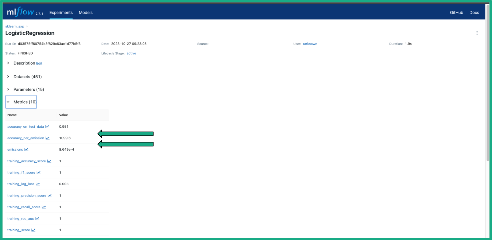
In the MLflow user interface, you'll find a range of standard metrics that are part of MLFlow, including well-known metrics like accuracy, F1-score, precision, recall, and others. These metrics are complemented by the emissions metrics we have discussed above.

Benchmarking Image recognition models using MLFlow-emissions-sdk

To test our newly created package, we preform a benchmarking of different pre-trained image recognition models. Comparing them using various metrics including the carbon emissions metrics we defined. We train the pre-trained models upon a Kaggle dataset containing 2527 images of garbage subdivided into six distinct categories (cardboard, paper, glass, metal, plastic and trash). In order to conduct a fair comparison of all the models we trained, we trained them on Google Collab using a NVIDIA T4 GPU. Since during the testing of the CodeCarbon package, we observed that it tracks the energy consumption of your local machine, which means it also considers other concurrently running processes. This can lead to skewed results.

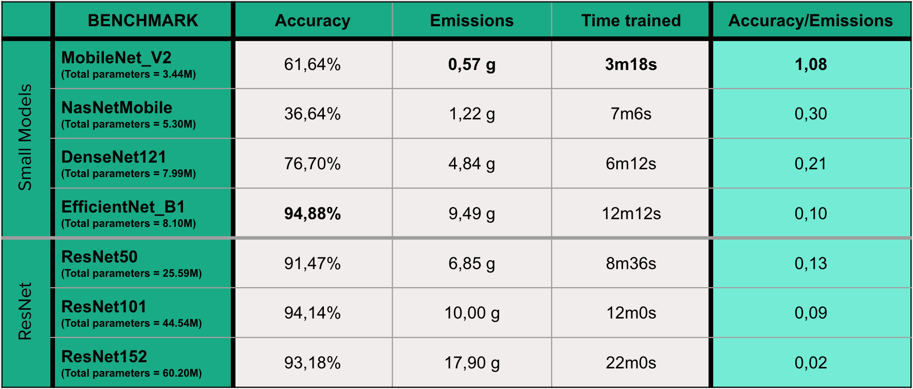
In the table below we have listed 7 different pre-trained image recognition models. Sorted from smalles to biggest model as measured by the number of parameters. NasNetMobile, MobileNetV2, DenseNet and EfficientNet are lightweight neural network models designed to run on edge devices, close to where the data is generated, rather than in a central cloud computing facility. They are considered edge AI models, which are becoming increasingly important as more and more devices are able to collect and process data at the edge. ResNet, or Residual Network, is a deep learning architecture that is commonly used for a variety of tasks, including image classification. While they can also be used as an edge AI model we put it in a separate category since these models are much larger than the rest. It is known for its ability to achieve high accuracy while being relatively efficient. The integer next to the ResNet model name indicates the number of residual blocks that the model contains. We compare them using the normal metrics included in MLFlow and the metrics we have defined ourself.

The EfficientNet model demonstrated exceptional accuracy, outperforming the more complex ResNet models. The ResNet models also achieved relatively high accuracy scores, which can be considered within the margin of error of the EfficientNet model's accuracy. Considering other metrics, MobileNet, the smallest model, emitted the least carbon, which can be partly attributed to its shorter training time. It is therefore unsurprising that MobileNet also achieved the highest score on the accuracy per emission metric by a significant margin.

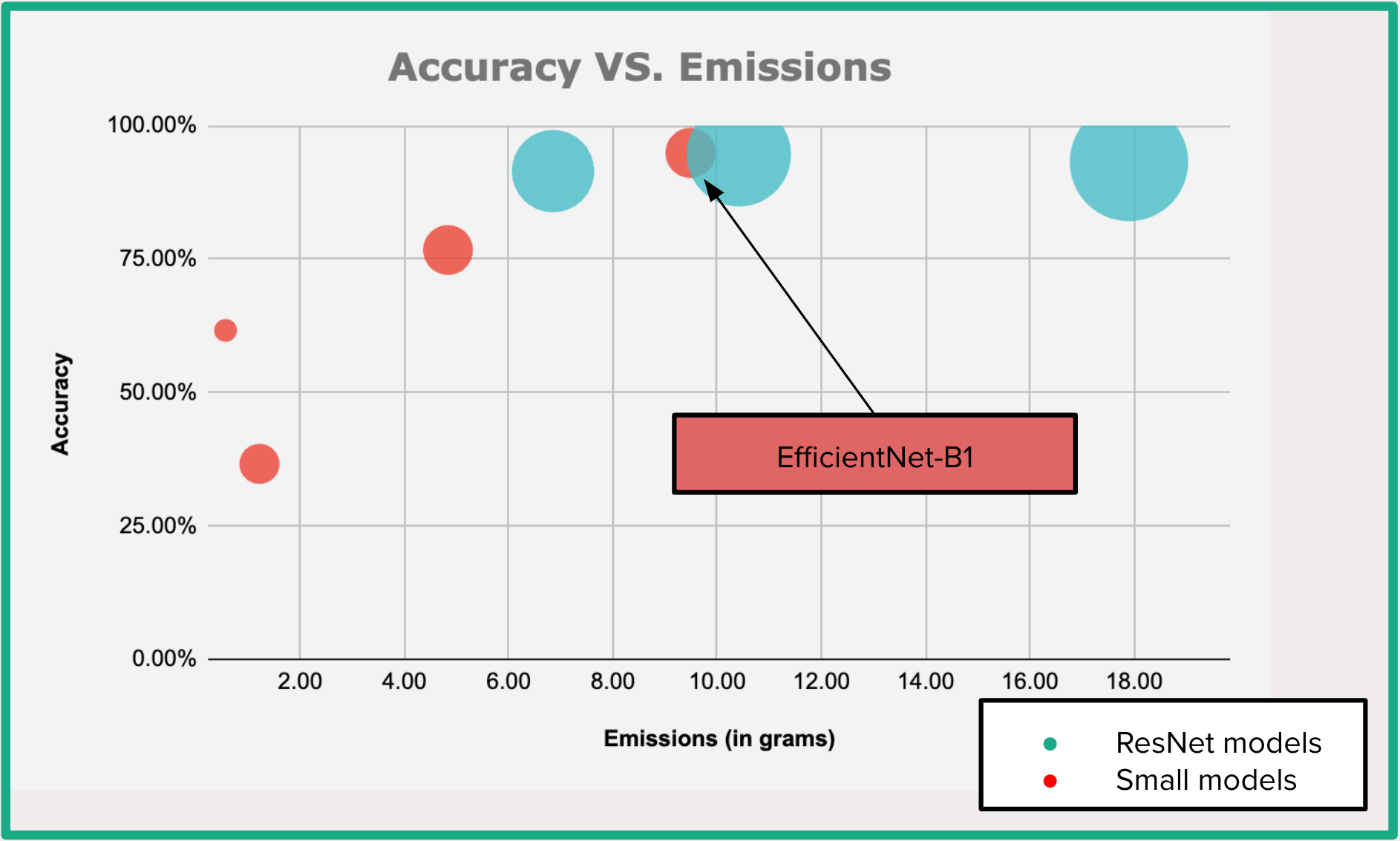
Another way to visualise these results is through a bubble scatter plot, in which the size of the bubbles represents the model size as measured by the total number of parameters.

Overal, the scatter plot illustrates a trade-off between accuracy and carbon emissions when deciding on a machine learning model. Opting for the EfficientNet or a ResNet model will provide the highest accuracy, whereas selecting a MobileNet model will be more environmentally friendly with lower carbon emissions. Nevertheless, it's important to note that the MobileNet model has a limited accuracy on this specific dataset.

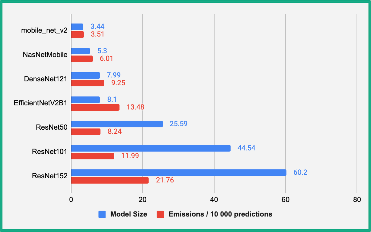
Additionally, our package incorporates the metric emission_per_10_inferences, which forecasts a model's carbon footprint upon deployment. To enhance the visualisation of this metric on the clustered bar chart below, we scaled it to 10,000 inferences.

The graph shows that there is a general trend of increasing emissions with increasing model size. However, there are some exceptions to this trend. For example, the EfficientNet_B1 model has a lower emissions per 10,000 predictions than the ResNet101 model, even though the EfficientNetV2B1 model is larger. This suggests that the efficiency of the model architecture also plays a role in determining emissions. More efficient models can achieve the same level of performance with fewer parameters and less computation, which results in lower emissions.

The full package is available on GitHub, including example notebooks with implementations of our model in Keras, PyTorch, and Sklearn ML applications. If you like our package, please consider giving it a star! Other comments or suggestions are also welcome.

Sources:

Strubell, E., Ganesh, A., & McCallum, A. (2019). Energy and policy considerations for deep learning in NLP. arXiv preprint arXiv:1906.02243.

https://www.iea.org/energy-system/buildings/data-centres-and-data-transmission-networks#programmes

Andrae, A. S., & Edler, T. (2015). On global electricity usage of communication technology: trends to 2030. Challenges, 6(1), 117-157.

Codecarbon.io. CodeCarbon.io. (2023). https://codecarbon.io/